Simulation based methods for time series diagnostics

University of London

Simulation-based methods for time series

diagnostics

Maria Teresa Catarino Leitao

London School of Economics and Political Science

A thesis su b m itted in fulfillment of th e requirem ents for obtaining th e degree of D octor of Philosophy

Department o f Statistics, Houghton Street, London WC2A 2 A E

UMI Number: U 615246

All rights reserved

INFORMATION TO ALL U SE R S

The quality of this reproduction is d ep en d en t upon the quality of the copy subm itted. In the unlikely even t that the author did not sen d a com plete m anuscript

and there are m issing p a g e s, th e se will be noted. Also, if material had to be rem oved, a note will indicate the deletion.

Dissertation Publishing

UMI U 615246

Published by ProQ uest LLC 2014. Copyright in the Dissertation held by the Author. Microform Edition © ProQ uest LLC.

All rights reserved. This work is protected against unauthorized copying under Title 17, United S ta tes C ode.

ProQ uest LLC

789 East E isenhow er Parkway P.O. Box 1346

A bstract

Acknowledgm ents

I would like to th an k my supervisor, Dr. Jerem y Penzer, for th e always useful advises. For sharing his knowledge w ith me and for th e perm an en t availability in helping me to overcome th e problem s th a t arouse in my PhD research, over these years. Dr. Jerem y Penzer encouraging words and confidence in my work had an essential role in keeping my m otivation to conclude this P h D thesis.

To Sim ona, an im m easurable th a n k you, difficult to express in words. For her friendship and com panionship since we have m et, b o th as PhD students. For being always there to listen to me. For listen to my never ending com plains, b u t also for sharing my happiness when things were going th e right way.

To my friends, in London and Portugal, in p articu lar P atricia, Isabel, Irini and B eatriz, a special th an k you for th eir friendship, in th e good and less good moments.

Above all I would like to th an k my family. My parents, for th eir love, confidence in my capacities and unconditional support. To my sister A n ita and my brother To, for being always so close to me, despite th e distance.

Contents

1 Introduction

15

2 Sim ulation m ethods for state space m odels

22

2.1 I n tr o d u c tio n ...22

2.2 M arkov chain M onte Carlo m e th o d s ... 24

2.2.1 Definitions and ergodic r e s u l t s ...24

2.2.2 M etropolis-H astings a lg o r ith m ...28

2.2.3 G ibbs s a m p le r ... 30

2.2.4 Some practical i s s u e s ...31

2.3 S tate space m o d e l s ... 32

2.4 M CMC m ethods for state space m o d e ls ... 39

2.4.1 Sim ulating f r o m / ( a | ^ , y ) ... 39

2.4.2 Sim ulating from f(Sfr\Y,ct) for th e BSM... ... 41

2.4.3 N um erical examples ... 44

2.5 C o n c lu s io n s ... 50

3

M CM C m ethods for shocks detection

52

3.2 Interventions in state space m o d e l s ...53

3.3 Non-Bayesian shock d i a g n o s i s ...56

3.4 Bayesian shock d ia g n o s is ...57

3.4.1 G ibbs sam pling assum ing a discrete prior for K t ...60

3.5 Generalizing the interventions prior d i s t r i b u t i o n ...65

3.5.2 D etection of outliers and level shifts w ith an uninform ative

prior for the shocks m a g n itu d e ... 78

3.5.3 A M onte Carlo s t u d y ...81

3.5.4 S tatio n ary model: AR(1) plus n o i s e ... 85

3.5.5 Em pirical application: coal consum ption d a ta s e t ... 87

3.6 C o n c lu s io n s ... 96

4 E stim ation of unobserved com ponent m odels in th e presence of

outliers and structural shifts

98

4.2 Unobserved com ponents model w ith intervention v a r i a b l e s ... 100

4.3 A M onte Carlo s t u d y ... 108

4.4 E m pirical application: m arriages d a ta s e t ...113

4.5 C o n c lu s io n s ... 122

5 D etection o f outliers and level shifts in unobserved com ponent

m odels w ith a null noise variance

123

5.2 Sam pling from the state space variable full conditional distrib u tio n . 127 5.2.1 Sam pling from N (0, W ) ...129

5.2.2 Sam pling from A ( E ( u |F ) ,v a r ( u |y ) ) ...130

5.2.3 G eneralization for including intervention v a r ia b le s ...131

5.3 D etection of outliers and level shifts when o \ — 0 ... 134

5.3.1 Sensitivity analysis to th e choice of erf ... 139

5.3.2 A M onte Carlo s t u d y ... 143

5.3.3 Em pirical application: bonds d a ta s e t ...145

5.4 D etection of outliers and level shifts when cr^ = 0 ...151

5.4.1 Sensitivity analysis to th e choice of a*...160

5.4.2 A M onte Carlo s t u d y ... 164

5.4.3 Em pirical application: Nile d a ta s e t ... 167

6 Conclusions

177

A Ox im plem entation o f th e Gibbs sampler for em pirical application

List of Tables

2.1 Sum m ary of o u tp u t from posterior sam ples for hyperparam eters, for a local level m odel... 44 2.2 Sum m ary of o u tp u t from posterior sam ple m eans for h yperparam ­

eters, across 1,000 sim ulated replications, for prior p aram eter Si = 1 .3 .5 and c\ = C2 = s 2 = 5, for a local level m odel... 47

2.3 Sum m ary of o u tp u t from posterior sam ple m eans for hyperparam ­ eters, across 1,000 sim ulated replications, for prior p aram eter $ 2 =

1 .3 .5 and C\ = c2 = S\ = 5, for a local level m odel... 47 2.4 Sum m ary of o u tp u t from posterior sam ple of hyperparam eters, for

1,000, 100,000 and 1,000,000 runs of the G ibbs sam pler , for tru e param eters a 2 = 1, a 2 = 0.1,0.01... 48 3.1 Sum m ary of o u tp u t from posterior sam ple m eans, for th e local level

m odel w ith intervention variables in th e m easurem ent equation, across 100 sim ulated replications, for th e norm al prior param eter a 2 = 1 0 ,2 0 ,5 0 ,1 0 0 ,2 0 0 ,5 0 0 ... 70 3.2 Sum m ary of o u tp u t from posterior sam ple m eans, for th e local level

m odel w ith intervention variables in th e m easurem ent equation, across 100 sim ulated replications, for the approxim ating uniform d istrib u ­ tion param eters V\ = 5 .5 ,7 .7 ,1 2 .2,1 7 .3 ,24 .5 ,3 8 .7 and u\ = —Vi. . . . 76 3.3 Sum m ary of o u tp u t from posterior sam ple averages, across 10,000

sim ulated replications, for a local level m odel... 84 3.4 Sum m ary of o u tp u t from posterior sam ple m eans of hyperparam eters,

3.5 Posterior average probability and size of outliers detected for the coal d a ta set, from 1960Q1 to 1984Q4...91 3.6 Sum m ary of o u tp u t from posterior samples of the hyperparam eters,

and prior probabilities of an outlier and a level shift, for th e coal d a ta set, from 1960Q1 to 1984Q4... 91 4.1 Sum m ary of o u tp u t from posterior sam ple m eans of hyperparam eters,

across 5,000 sim ulated replications, for BSM ... 110 4.2 Sum m ary of o u tp u t from posterior sam ple m eans for intervention

variables, across 5,000 sim ulated replications, for BSM ... I l l 4.3 Sum m ary of o u tp u t from posterior sample of interventions variables

for stru c tu ra l shifts detected for the m arriages d a ta set, from 1958Q1 to 1984Q4... 116 4.4 Sum m ary of o u tp u t from posterior sample of hyperparam eters, for

th e m arriages d a ta set, from 1958Q1 to 1984Q4...117 4.5 Variance-covariance m atrix of posterior sam ples of hyperparam eters,

for th e m arriages d a ta set, from 1958Q1 to 1984Q4... 119 5.1 Sum m ary of o u tp u t from posterior sam ple averages, across 500 sim­

ulated replications, obtained from application of stage 1 of sampling scheme 5.1, for erf = 0 .2 5 ,0 .5 ,1 ,2 ... 140 5.2 Sum m ary of o u tp u t for posterior sample averages, across sim ulated

replications, obtained from application of stage 2 of sampling scheme 5.1, for a f = 0 .2 5 ,0 .5 ,1 ,2 ... 142 5.3 Sum m ary of o u tp u t from posterior sam ples averages, across 5,000

sim ulated replications, for a local level m odel w ith o f = 0 ... 144 5.4 Sum m ary of o u tp u t from posterior samples of intervention variables

for outliers and level shifts detected, for th e bonds d a ta set, from 1916-8 to 1930-6... 151 5.5 Sum m ary of o u tp u t from posterior sam ples of th e hyperparam eters,

5.6 E stim atio n results by m axim um likelihood, given th e position of the

shocks, for th e bonds d a ta set, from 1916-8 to 1930-6... 156 5.7 Sum m ary of o u tp u t from posterior sam ple averages, across 500 sim­

u lated replications, obtained from application of stage 1 of sampling scheme 5.2, for cr^* = 0 .2 5 ,0 .5 ,1 ,2 ...162 5.8 Sum m ary of o u tp u t from posterior sam ple averages, across sim ulated

replications, obtained from application of stage 2 of sampling scheme 5.1, for = 0 .2 5 ,0 .5 ,1 ,2 ...164 5.9 Sum m ary of o u tp u t from posterior sam ples averages, across 5,000

sim ulated replications, for a local level m odel w ith cr^ = 0... 166 5.10 Sum m ary of o u tp u t from posterior sam ples, for th e Nile d a ta set,

from 1871 to 1970... 171 5.11 E stim atio n results by m axim um likelihood, given th e position of the

List of Figures

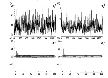
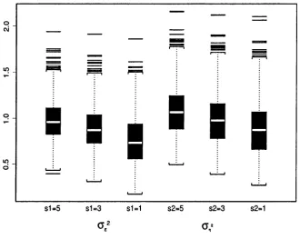
2.1 P lo t of sim ulated p a th s (a)-(b), and autocorrelation functions for posterior samples (c)-(d), for <r2 and cr2, for a local level model. . . . 45 2.2 Box-plots of posterior sam ple means of hyperparam eters, across 1,000

sim ulated replications, for prior param eters {si = 1 ,3 ,5 , c\ = C2 = S2 = 5}

and { $ 2 = 1? 3,5 , Ci = C2 = si = 5}, for a local level m odel... 46

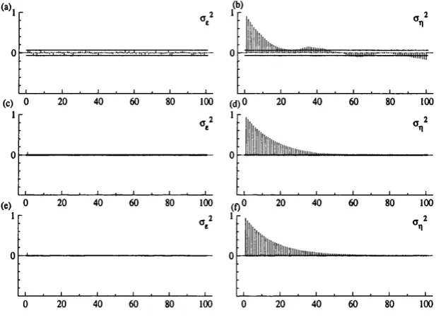
2.3 A utocorrelation functions for posterior sam ples of th e hyperparam e­ ters for a local level model, w ith tru e param eters o \ — 1, <r2 = 0.01, for 1,000 (a)-(b), 1000,000 (c)-(d) and 1,000,000 (e)-(f) runs of the G ibbs sam pler... 49 2.4 A utocorrelation functions for posterior sam ples of th e hyperparam e­

ters for a local level model, w ith tru e param eters o f = 1, a2 — 0.1, for 1,000 (a)-(b), 1000,000 (c)-(d) and 1,000,000 (e)-(f) runs of the G ibbs sam pler... 50 3.1 Shocks in sta te space models: simple additive outlier (a); innovative

outlier in statio n ary AR(1) (b); level shift (c); seasonal shift (d). . . . 55 3.2 Box-plots of posterior m ean size of outlier, across 100 sim ulated repli­

cations, for norm al prior param eter <j2 = 1 0 ,2 0 ,5 0 ,1 0 0 ,2 0 0 ,5 0 0 , for

a local level m odel...71 3.3 Box-plot of posterior m ean size of outlier, across 100 sim ulated repli­

3.4 A rtificial d a ta set generated from a local level model, w ith T = 100, w ith outliers a t tim e t — 20 and t = 50, of size 7 and -6, and level shifts a t tim e t — 40 and t = 75 of size 7 and -7 ... 82 3.5 Box-plot of posterior sam ple m eans of probability of outliers (a)-(b)

and level shifts (c)-(d), across 10,000 sim ulated replications, for a local level m odel...83 3.6 H istogram s (a)-(b) and and box-plots (c)-(d) of posterior sam ple

m eans of hyperparam eters, across 10,000 replications, for a local level m odel... 83 3.7 P lots of posterior m eans of indicator and size of intervention variables

for outliers (a)-(b) and level shifts (c)-(d), for AR(1) plus noise model. 86 3.8 S catter plot of posterior samples for (o f, o f) (a), cross correlations

(b), autocorrelation functions (c)-(d) for posterior sam ples of hyper­ param eters until lag 100, for AR(1) plus noise m odel...86 3.9 Q uarterly coal consum ption (logarithm ), in th e UK, from 1960 quar­

te r 1 to 1986 q u arter 4 ... 87 3.10 P lots of posterior means of indicator and size of intervention variables

for outliers (a)-(b) and level shifts (c)-(d), for th e coal d a ta set, from 1960Q1 to 1986Q4... 89 3.11 A utocorrelation functions for posterior sam ples for o f and o f, for 50

lags, for the coal d a ta set, from 1960Q1 to 1986Q4...92 3.12 S catter plots of posterior samples for size of intervention variables of

outliers detected, for the coal d a ta set, from 1960Q1 to 1986Q4. . . . 93 3.13 A utocorrelation functions for posterior sam ples for size of intervention

variables of outliers detected , for 500 lags, for th e coal d a ta set, from 1960Q1 to 1986Q4... 94 3.14 D escriptive plots of standardized innovations, for th e coal d a ta set,

from 1960Q1 to 1986Q4... 95 3.15 P lots (a)-(b) and box-plots (c)-(d) of standardized auxiliary residuals,

4.1 Artificial d a ta set generated from BSM w ith outlier, level, slope and seasonal shifts... 109 4.2 H istogram s (a)-(d) and box-plots (e)-(f) of posterior m ean estim ates

of hyperparam eters, across 5,000 sim ulated replications, for BSM. . . 110 4.3 H istogram and box-plot of estim ates of m agnitude of outlier (a)-(b),

level shift (c)-(d), slope shift (e)-(f), seasonal shift (g)-(h), across 5,000 sim ulated replications, for BSM ...112 4.4 Q uarterly num ber of m arriages in the UK from 1958Q1 to 1984Q4 . . 114 4.5 P lots of posterior means of indicator and size of intervention variables

for level shifts (a)-(b) and seasonal shifts (c)-(d), for th e m arriages d a ta set from 1958Q1 to 1984Q4...116 4.6 H istogram s (a)-(d) and box-plots (e)-(f) of posterior sam ples of hy­

p erparam eters, for the m arriages d a ta set, from 1958Q1 to 1984Q4. . 117 4.7 A utocorrelation functions for th e posterior sam ples of hyperparam e­

ters, for 1,000 lags, for the m arriages d a ta set, from 1958Q1 to 1984Q4.118 4.8 S catter plots of the posterior samples of hyperparam eters, for the

m arriages d a ta set, from 1958Q1 to 1984Q4... 119 4.9 D escriptive plots of standardized innovations, for th e m arriages d a ta

set, from 1958Q1 to 1984Q4... 120 4.10 P lots of standardized auxiliary residuals, for m arriages d a ta set, from

1958Q1 to 1984Q4... 121 5.1 Box-plots of posterior sample m eans of size of outlier, across 500

sim ulated replications, for erf = 0 .2 5 ,0 .5 ,1 ,2 ... 141 5.2 H istogram s, and box-plots of estim ates of size of outlier (a)-(b) and

level shift (c)-(d), across 5,000 sim ulated replications, for a local level m odel w ith o f = 0... 146 5.3 M onthly quotes of Greek Government bonds from A ugust 1916 to

June 1930... 147 5.4 P lots of posterior means of indicator (a) and size (b) of an outlier,

5.5 P lots of posterior means of indicator (a) and size (b) of level shift, for bonds d a ta set, from 1916-8 to 1930-6... 150 5.6 H istogram and box-plot of posterior sample for size of outlier detected

in 1923-3, for th e bonds d a ta set, from 1916-8 to 1930-6... 152 5.7 H istogram s and box-plots of posterior samples for size of level shifts

detected in 1919-12 (a)-(b), 1922-2 (c)-(d), 1922-11 (e)-(f) and 1923-2 (g)-(h), for th e bonds d a ta set, from 1916-8 to 1930-6... 153 5.8 Descriptive plots of standardized innovations, for bonds d a ta set, from

1916-8 to 1930-6... 154 5.9 P lots (a)-(b) and box-plots (c)-(d) of standardized auxiliary residuals,

for bonds d a ta set, from 1916-8 to 1930-6... 155 5.10 Box-plot of posterior samples m ean of size of level shift, across 500

sim ulated replications, for = 0 .2 5 ,0 .5 ,1 ,2 ...163 5.11 H istogram s and box-plots of estim ates of size of level shift (a)-(b)

and outlier (c)-(d), across 5,000 sim ulated replications, for local level m odel w ith = 0... 167 5.12 A nnual volume of the river Nile a t Aswan, between 1871 and 1970. . 168 5.13 P lots of posterior means of intervention variables for th e presence of

a level shift (a)-(b), and for the presence of an outlier (c)-(d), for the Nile d a ta set, from 1871 to 1970... 169 5.14 H istogram s and box-plots of posterior samples for size of level shift

detected in 1899 (a)-(b) and outliers detected in 1877 (c)-(d), 1888 (e)-(f), 1913 (g)-(h) and 1964(i)-(j), for the Nile d a ta set, from 1871 to 1970... 173 5.15 D escriptive plots of standardized innovations, for th e Nile d a ta set,

from 1871 to 1970... 175 5.16 P lots (a)-(b) and box-plots (c)-(d) of standardized auxiliary residuals,

Chapter 1

Introduction

A tim e series is a sequence of observations recorded over tim e. In general, th e obser­ vations are serially correlated. T he purpose of m odeling tim e series is to determ ine th e stru ctu re th a t best explains this correlation, and use it to forecast th e future behaviour of th e series.

For sta te space models, th e observations evolve over tim e as a linear function of a sta te variable. T he s ta te variable is often laten t. S ta te space m odels are widely used after th e K alm an filter was proposed in K alm an (1960). These models present a high degree of flexibility in th e type of dynam ics they can model. For example, any linear tim e series process has a sta te space representation.

S tru ctu ral models are a class of unobserved com ponents models. T hey decompose th e tim e series in th e sum of several unobserved effects, com m only irregular, trend, seasonal or cyclical effects. S tru ctu ral models fit n a tu ra lly into th e sta te space framework. In Harvey (1989), an extensive stu d y of th e properties an d algorithm s for stru c tu ra l tim e series is presented. The basic stru c tu ra l m odel is defined as consigning irregular, tren d and seasonal com ponents.

m ore persistent effect results in a stru c tu ra l shift. One of th e first characterizations of shocks in tim e series m odels is given in Fox (1972).

Bayesian m ethods for estim atin g tim e series models, are based on th e statistical properties of the posterior sam ples of th e param eters of th e model. The semi­ nal work of M etropolis, R osenbluth, R osenbluth, Teller, and Teller (1953) draws a tte n tio n to th e po ten tial statistic a l applications of these m ethods and lay the foundations for Markov chain M onte Carlo techniques. As access to com puters is w idespread and more powerful machines are available, th e p o p u larity of Bayesian techniques has increased. Bayesian m ethodologies in tim e series are well established and have accum ulated a large literature. One of th e m ore frequently used tools is the M etropolis-H astings algorithm (H astings, 1970). T he G ibbs sam pler, Gem an and G em an (1984), which can be viewed as a com position of several M etropolis-H astings steps, is the technique we shall focus our atte n tio n on.

T he aim of this work is to derive and im plem ent sam pling-based m ethods for the estim ation of stru c tu ra l tim e series, in th e presence of outliers an d stru c tu ra l shifts. O ur contribution has three m ain components:

• th e prior d istrib u tio n for th e size of th e shocks variable use of a flat uninfor­ m ative distribution.

• a Bayesian m ethodology for the estim ation of a basic stru c tu ra l m odel (BSM), in th e presence of outliers, level shifts, slope shifts and seasonal shifts.

• a Bayesian m ethod for th e detection of outliers and level shifts, for a local level model, when one of th e hyperparam eters is equal to zero, assuming a continuous prior distrib u tio n for the size of th e shocks variables.

th a t m ight be present in the d ata. W hen assum ing a m ultinom ial prior, we have to define a priori th e set of values from which to sam ple th e size of th e shocks. Assum ing a norm al d istribution, th e prior m ean and variance are set a priori. We show th a t th e posterior samples obtained for th e size of th e shocks variables, present some undesirable sensitivity to th e choice of the d istrib u tio n param eters, nam ely to th e choice of th e variance. A ssuming a flat prior d istrib u tio n , th e param eters u and

v for a U [u, v] have to be set a priori. We show, by m eans of a sensitivity study, th a t th e posterior samples present less sensitivity to th e choice of these param eters, th a n to the choice of th e norm al distrib u tio n param eters. Therefore, by assuming a uniform d istrib utio n we ob tain an estim ation m ethod th a t is less dependent on prior assum ptions th a n the existent methodologies.

Generalizing th e m ethod we propose for detecting outliers and level shifts, we present a Bayesian algorithm for detection of outliers and stru c tu ra l shifts, for th e basic stru c tu ra l model. The BSM defines the dynam ics of a tim e series as th e sum of several com ponents: an irregular, tren d and seasonal com ponent. We consider th e case of a tren d w ith a stochastic slope com ponent. Given this decom position of the tim e series, two m ain types of shocks m ight occur: outliers and stru c tu ra l shifts. The stru c tu ra l shifts can be of three types: level, slope and seasonal shift. We form ulate a m odel allowing for these four type of shocks. Using th e G ibbs sam pler, we estim ate th e hyperparam eters and sim ultaneously detect th e position and estim ate the size of shocks in th e d ata. An additional innovation is th a t we assum e a uninform ative uniform prior for the size of all th e type of shocks considered. T he choice of this prior distrib u tio n has th e aim of m aking the process of detection and characterization of th e shocks has independent as possible, from prior knowledge of th e behaviour of th e tim e series data.

being equal to zero is often overlooked in th e literatu re. G erlach, C arter, and Kohn (2000), deal w ith this case, b u t they assum e a discrete prior d istrib u tio n for the intervention variables. As we have argued before, th is assum ption is restrictive and dem ands a considerable prior knowledge of th e d a ta set.

To overcome th e problem posed by having one of th e hyperparam eters equal to zero in th e uniform prior case, we propose a two stage sam pling scheme. In the first stage we apply th e G ibbs sam pler to an auxiliary d a ta set. T his d a ta set is constructed in such a way th a t it has the sam e shocks as the original d a ta set. It is modeled as a local level model, b u t w ith b o th hyperparem eters different from zero. It is used to detect the shocks, th a t affect th e observations th ro ug h th e equation w ith th e null hyperparam eter. In the second stage, we ru n a second G ibbs sam pler to detect th e other type of shocks and estim ate th e non null hyperparam eter.

T he results presented for th e em pirical applications and M onte C arlo studies are obtained using Ox (Doornik, 1999). The Ox package SsfPack, (K oopm an, Shephard, and D oornik, 1999), for estim ation of state space m odels, was also used extensively. T he results obtained using m axim um likelihood, which are rep o rted for comparison w ith th e results we obtain by using our Bayesian approach, were generated using the stru c tu ra l tim e series package STAMP (K oopm an, Harvey, D oornik, and Shephard,

2000).

prior distributions of th e hyperparam eters, on th e param eters estim ated.

In C h ap ter 3 we study the detection of outliers and level shifts, for th e local level m odel, using th e Gibbs sampler. We assum e th a t b o th hyperparam eters are different from zero. The model is form ulated for th e detection of shocks by including intervention variables for the presence of outliers and level shifts. For each type of shock th is am ounts to defining two intervention variables: an ind icato r variable for th e presence of a shock, and a size of shock variable. T h e innovation in th e m ethod we propose is th a t the size of th e shock is assum ed to have a flat prior distribution. W hen assum ing a flat distribution, th e boundaries of a bounded uniform d istrib u tio n have to be set a priori. To compare the perform ance of th e sam pler when assum ing a flat prior w ith a norm al prior for the size of th e shocks variable, we perform an analysis of sensitivity to the choice of th e p aram eters of th e norm al and uniform distributions. We show th a t using th e flat prior, th e estim ation results are less sensitive to the choice of th e prior d istrib u tio n param eters. H aving established th e benefits of th e uninform ative prior, a sam pling alg o rithm is proposed for estim ating a local level model, in the presence of outliers and level shifts. A M onte C arlo study is presented, for assessing the perform ance of th e sam pler. T he artificial d a ta sets are generated from a local level model, where two outliers and two level shifts are in p u t. To illu strate th e application of the m eth o d to a real d a ta set, we consider th e d a ta com posed of th e coal consum ption in th e UK, from th e first q u a rte r of 1960 to th e fourth qu arter of 1986.

different from zero. O ur contribution, is th a t we present a m eth o d for sim ultaneously estim ate th e hyperparam eters and detect any type of shock, for a basic stru ctu ral m odel. Furtherm ore, w ith the uniform prior assum ptions th e shock detection is done w ithout requiring an extensive prior analysis of th e d a ta. T he results from a M onte Carlo study are presented. The d a ta are generated from a basic stru ctu ral model. All th e four type of shocks are in p u t to each d a ta set: an outlier, a level shift, a slope shift and a seasonal shift. O ur m ethodology is applied to th e real d a ta set of th e num ber of marriages in the UK, from th e first q u a rte r of 1958 to the fourth q u arter of 1984.

run, for th e original d a ta set. It delivers an estim ate for th e irregular variance, th e position of th e outliers and estim ates of th eir sizes. T he perform ance of the sam pling schemes proposed is analyzed by two M onte C arlo studies, for each of th e hyperparam eters equal to zero. As an em pirical application, when th e irregular variance is equal to zero, we m odel the real d a ta set of m onthly quotes of bonds issued by th e Greek government, from A ugust 1916 to June 1930. T he volume of th e Nile d a ta set, from 1871 to 1970, is used as an em pirical application, for the case when th e level variance is equal to zero.

Chapter 2

Sim ulation m ethods for state

space models

2.1

Introduction

A broad lite ra tu re is available on classical m ethods for estim atin g param etric tim e series models, from ARMA models, (Box and Jenkins, 1970) to state space models (SSM), (Harvey, 1989). The aim of this chapter is to review Bayesian m ethodologies for estim ating tim e series which fit in th e space s ta te m odeling framework.

T he basic difference between Bayesian and classical approaches for param etric inference is th a t Bayesian m ethods make no d istin ctio n betw een observations Y

and param eters 9, in th a t they consider all of th em random variables. P aram etric inference is based on th e posterior distribution P ( 9 \Y ) . M eans, quantiles, confidence intervals or any other statistical properties for 9 are obtained from sam ples of th a t posterior. In m ost cases the posterior d istrib u tio n is n o t available in a closed form; th e m ethodology used to overcome this problem is w h at distinguishes th e m ajority of Bayesian m ethods.

T he im pact of th e param eters on the observable Y is m easured by th e likelihood function P ( Y \9 ). Inform ation, if any, on the p aram eters distrib u tio n previous to th e observation of Y is sum m arized in th e prior distribution P (9). Using Bayes’ theorem we have the following expression th a t relates these th ree distributions:

p(e)P(Y\e)

J P ( 0 ) P ( Y \ 0 ) d 0 ' ( ' 1

(2.1) states th a t th e posterior distribution P { 0 \Y ) is p roportional to th e product of th e likelihood P ( Y \ 6), and th e prior distrib u tio n P(0):

P ( 9 \Y ) oc P ( 9 )P ( Y \6 ).

M arkov chain M onte Carlo (MCMC) m ethods rely on constructing a process which is M arkovian and has as its lim iting d istrib u tio n th e posterior distribution. M CM C m ethods are distinguished by th e way in which these processes are con­ stru cted . W hen applying this m ethodology to tim e series, Y will be a set of tim e series d a ta { Y i, . . . , Yt} and 9 the set of param eters in th e model, together w ith any m issing observations.

In section 2.2 th e m ain Markov chain notations will be presented, together with results th a t are the basis for MCMC m ethods. T he characterization of these m ethods will be done w ith special reference to th e M etropolis-H asting algorithm and the G ibbs sam pler. Com m ents are m ade on problem s arising in th e use of th e general MCMC framework.

T he m ain objective of the results presented for M CM C m ethods is th eir applica­ tion to SSM. These models are introduced in section 2.3, together w ith examples, and algorithm s.

For simplicity, we consider the estim ation of SSM, in th e context of th e Gibbs sam pler, divided in two steps: sam pling from th e full conditional of th e state vector and sam pling from th e full conditional of the param eters. To sam ple from the full conditional of th e states we use a sim ulation sm oother algorithm , and th is m ethod is explained for a general SSM. T he m ethodology for sam pling from th e full conditional of th e param eters is presented for an unobserved com ponents m odel (UCM).

2.2

M arkov chain M onte Carlo m eth od s

2.2.1 D efin ition s and ergodic results

A sequence of random variables . . . , X ^ \ . . . is a Markov chain (X ^ if th e d istrib u tio n of given all th e previous states of th e chain . . . , X ®

depends only on X ® . For any t,

P ( a (‘+1) G A |A (0), X (1), . . . , X (t)) = P ( A (m ) G A |A (t)) ,

for any given A G B (S'), the set of all th e subsets of S, th e sta te space where th e chain is defined. Typically A is a subset of 9ft*. T he transition kernel P ( x , A ) of a Markov chain is defined as:

P ( x , A ) = P { x (,+1) € A \ X<*> = i } . (2.2) We are interested only in tim e homogeneous M arkov chains and for th a t reason

P ( x, A) in (2.2) is independent of t.

T he n th -ite ra te of (2.2) is

P n (x, A ) = P { x (n) 6 = X} ,

and P " (-|x ) th e conditional distribution of given th e in itial sta te of the chain

X ^ = x .

A d istrib u tio n ir is an invariant distribution for a M arkov chain if: »(A ) = / P ( x , A ) n (x )d x ,

for all m easurable sets A. Under certain general conditions, which are stated later, an invariant d istrib u tio n 7r is also an equilibrium distrib u tio n , th a t is, for 7r-almost

x 1:

lim P n ( x ,A ) — >7r(A),

n-Aoo v \

In other words, under some conditions, if we run th e chain for long enough, th e d istrib u tio n of th e states converges to the invariant d istrib u tio n independently of th e in itial state distribution.

Suppose we w ant to estim ate E n (g):

E* (9

) = J

where #(•) is a real-valued function. If we construct a M arkov chain ( X ^ ) th a t converges to th e ta rg e t distribution 7r(-), th e sam ple analogue to th e expectation in (2.3) is:

= = (2 -4)

iV i= 1

In order to be able to use Markov chains so th a t (2.4) converges to th e expected value in (2.3) several questions m ust be addressed. In p articu lar, we require conditions

%

th a t insure convergence of th e chain to a unique lim it d istrib u tio n , and a m ethod to construct th e desired chain. We s ta rt by presenting some general definitions and results for M arkov chains. Afterwards we explain some of th e m ethods available for constructing those chains, which are a subset of th e available M CM C techniques.

Let P be th e tran sitio n kernel of a M arkov chain, defined in a finite cr-algebra

( S , B ( S ) ) . Given a cr-finite measure 7r, P is it-irreducible if, independently of the in itial state X ^ ° \ the probability of achieving any m easurable set A G B ( S), w ith 7t(A) > 0, in a finite num ber of steps is positive; th a t is, for each x G S there exists an n such th a t P n(x, A) > 0.

An 7r-irreducible chain is called r ec u rre n t if it will visit A an infinite num ber of times: for any m easurable set A w ith 7r(A) > 0,

P ( X G A infinitely often| = x) > 0 for all x, P ( X ^ G A infinitely often| = x) = 1 for 7r-almost x.

If P ( X ^ G A infinitely often | = x) = 1, for all x, th e chain is called

Harris recurrent.

A recurrent 7r-irreducible chain is positive recurrent if th ere is a finite invariant m easure for P . O therw ise th e chain is null recurrent.

and th ere exists n > 2 and a sequence of non-em pty sets {Ao, A i, . . . , A n-1} in B ( S )

such th a t for all i = 0 , . . . , n — 1 and all x E Af.

P ( x, Aj ) = 1, for j = i + 1 (m od n).

M CM C m ethods rely on constructing M arkov chains where th e invariant distri­ butio n coincides w ith th e ta rg e t distribution 7r. If th e chain is irreducible, positive recurrent and aperiodic th e next theorem , in T ierney (1994), implies th a t 7r is also

th e equilibrium distribution:

T h e o r e m 2 .2 .1 Suppose P is tt-irreducible and ir is an invariant distribution for P . Then P is positive recurrent and n is the unique invariant distribution o f P . I f P is also aperiodic then, fo r tt-almost x,

\\Pn{ x , . ) - 7 r \ \ T V ^ 0. (2.5)

I f P is Harris recurrent, then the convergence occurs fo r all x.

T he Total Variation distance || • ||tv is defined, for any bounded m easure <^> on

(S, B(S)), as

W^Wt v = sup <i>{A)- in f 6 (A )

AeB(S) AeB(S)

By defining a kernel w ith invariant d istrib u tio n 7r, such th a t it is irreducible, positive recurrent and aperiodic, after a long enough ru n of th e chain, states from th e equilibrium distrib u tio n 7r will be generated, independently from th e startin g state. T he question of how long should th e chain be ru n for is related to th e rate of convergence of (2.5) and will be addressed later. In order to present results concern­ ing th e asym ptotic properties of th e estim ator in (2.4) we s ta rt by presenting some definitions of ergodicity. A M arkov chain is called ergodic if it is H arris recurrent and aperiodic. A stronger form of ergodicity, is uniform ergodicity. A Markov chain is uniformly ergodic if th ere exists a constant M > 0 and 0 < r < 1 such th a t:

sup IIP n(x, •) - 7r||rv < M r 71, xex

T h e o r e m 2 .2 . 2 Suppose ( X ® ) is uniformly ergodic with equilibrium distribution 7r and suppose g is a real valued function and E 7r(g2) < oo. Then there exists a real number a(g) such that the distribution of

V N (

9

converges in distribution to a normal distribution with mean 0 and variance cr(g)2 fo r any initial distribution.

By construction, if is a random sam ple obtained from a statio n ary Markov chain, after convergence is achieved, all the X ® will have the sam e distribution, bu t they are not independent. A nd although th a t does not affect th e ergodic result in Theorem 2.2.2, it will have im plications in obtaining a consistent estim ato r of the variance <r(g)2, th e M CMC variance of th e posterior sam ple m ean. From th e tim e series literatu re a m ethod to obtain a consistent estim ate of th e variance for a correlated sam ple is by using a sm oothed estim ate of th e periodogram a t frequency 0, w ith an appro p riate choice of a lag window, see for exam ple Brockwell and Davis (1991).

Suppose we are interested in estim ating E v (g) where g G L 2 2, using a sim ulated sample . . . , from a Markov chain, which has reached equilibrium , by the sam ple m ean g n using th e form ula in (2.4). For estim atin g th e variance of gjq we use a Parzen window iu(*), defined as in Priestley (1981), in th e following way:

var (gN) = j j (2 .6 )

where

The bandw idth is chosen according to th e size of th e sam ple being considered and its correlation stru ctu re . T he weights of th e Parzen window are defined as:

w (x) =

1 — 6|z| 2 + 6 |z |3, |rc| < | , 2 ( 1 - |x |)3, \ < |ar| < 1,

0, otherwise.

\ 7

In Geyer (1992) several other m ethods for consistent estim atio n of th e MCMC vari­ ance are discussed.

T he relative numerical efficiency, Geweke (1989), is defined as th e ratio between th e lag window estim ator of th e variance and th e estim ate of th e variance if assum ing an independent sample. This quantity is a m easure of th e speed of th e m ixing of the chain.

In th e next section we see how th e previous results can be applied when consid­ ering M arkov chains constructed using the M etropolis-H astings algorithm and the G ibbs sam pler.

2.2.2

M etrop olis-H astin gs algorithm

T he M etropolis-H astings algorithm was proposed by H astings (1970). Suppose we are interested in sam pling from a targ et distrib u tion 7 r ( - ) , and th a t is easy to sample

from a proposal d istribution q(x\y), known up to a norm alizing constant. A Markov chain is constructed by using as generator density q ( y \ x ^ ) t where x ® is th e present sta te of th e chain. Let Y ~ q{y\x^ ) . The new sta te of th e chain will be given by:

w ith r(x ) = f a { x , y ) q ( y \ x ) d y .

In order to ensure th a t the ta rg e t d istribution 7r is also th e invariant distribution

of th e chain, a m inim al condition is imposed:

Y, w ith probability a { x ^ \ Y )

x ^ \ w ith probability 1 — a ( x ^ \ Y ), (2.7)

where

mm

T he tran sitio n kernel of the chain constructed in th is way is given by:

P (y \x ) = a { x, y)q(y\x) + (1 - r (x )) Sx (y)

U supp q{-\x) D supp 7r = <S,

x6 s u p p 7T

T h e o r e m 2 .2 .3 For every conditional distribution q, whose support includes S , ir

is an invariant distribution of the chain produced by (2.7).

T he following result, in R oberts and Tweedie (1996), gives sufficient conditions for irreducibility and aperiodicity of th e Markov chain obtained through th e M etropolis- H astings algorithm (assum ing S is connected):

T h e o r e m 2 .2 .4 Assum e 7r is bounded and positive on every compact set of its sup­ port S . I f there exist positive numbers e and 5 such that

q (y \x ) > e i f \x - y\ < 6,

then the Metropolis-Hastings Markov chain ( x ® '} is n-irreducible and aperiodic. Moreover, any nonem pty compact set is a small set.

Using Theorem 2.2.1, th e two previous theorem s provide sufficient conditions for the

M etropolis-H astings chain to converge to a unique lim it d istrib u tio n , th a t coincides w ith th e ta rg e t d istrib utio n 7T.

T he next theorem (see R obert and Casella, 1999 for proof), states conditions th a t ensure convergence of th e posterior sam ple m ean estim ator.

T h e o r e m 2 .2 .5 Suppose that fo r the Metropolis-Hasting Markov chain ( x ^ ) , we have that q{y\x) > 0 fo r every (x ,y ) € E <S x S (sufficient condition fo r being irre­ ducible).

I f g E L 1, then

lim gN = E n (g)

Tv— > 0 0

fo r 7r-almost everywhere.

These results do not provide any inform ation regarding th e ra te of convergence of th e chain. T h a t is an im p o rtan t aspect as the chain m ay rem ain in th e same state for a long tim e. The proportion of tim e t for which X (t+1) = X W is defined as the rejection rate.

Teller, and Teller, 1953), where q ( X \ Y ) = q ( Y|X ), and th e G ibbs sam pler (Ge­ nian and G em an, 1984, Gelfand and Sm ith, 1990) where th e proposal d istribution coincides w ith th e full conditional distribution.

2.2.3

G ibbs sam pler

Suppose th a t X ~ 7r(-), is composed of several blocks X = ( X i , . . . , XP) , p > 2. A dditionally suppose th a t it is possible to sam ple from all th e full conditional dis­ trib u tio n s 7u ( X i \ X - i ) , where X_* = ( X i , . . . , X j _ i , X i+i , .. . ,X P), for % = 1 , . . . ,p.

Let

X®

it will move, w ith probability one, to th e state X ^ t+1\ sequentially generated by:

X |t+1) ~ TTi (XilXi1?) ,

= l , . . . , p .

This algorithm generates a Markov chain w ith tran sitio n kernel:

p

P(y\x)

= n » (jfckj.

j

> *.

Vj, j < i)

i= 1

It is easy to check th a t th e u p d atin g of each com ponent can be done by application of th e M etropolis-H astings algorithm . Consider th e u p d a tin g of th e com ponent

i, x f \ Let 7T-i (•) be th e distrib u tion for th e vector X _j. A candidate Y* for the

u p d atin g of

X®

a Y v W v W n

. ( A Y u X ^ l M X h X ^ ) \

= m i n ( l , 1 ) = 1 .

= m in I 1

In conclusion, th e G ibbs sam pler is obtained by com posing several M etropolis- H astings algorithm s, w ith acceptance rates uniform ly equal to one and such th a t for each of those algorithm s the proposal d istributions are th e full conditional dis­ tributions.

By construction th e chain obtained w ith th e G ibbs sam pler has 7r as an invariant

th e full conditional distributions are not irreducible and so we can no t use the result in T heorem 2.2.1. In general to ensure th a t the chain is 7r-irreducible and aperiodic

is sufficient th a t:

,K i(X i\X -i) > 0, for all i and X , (2.8)

as is proved in G em an and G em an (1984) and C han (1993). U nder very mild conditions (R oberts and Sm ith, 1994), nam ely th e condition in (2.8) th e following convergence and ergodic results hold:

Convergence in distribution: As t —>• oo

( x ^ , x ' ( ) . . . , x < ‘>) 4 7T ( X u x 2 . . . , X„)

and hence for each i = 1, . . . , p

( X ^ ) 4 7Tj (Xi)

Geometric rate o f convergence:

Using th e T otal V ariation norm || • \\t v i ( X i \ x ! p . . . , X ^ converges to the tru e

d istrib u tio n in a geometric ra te of convergence in t.

Ergodic theorem: For any m easurable function T of ( X i , X 2 . . . , X p) whose expec­ ta tio n exists,

J im ~ g T ( X ? \ X<‘>. . . , X W ) “4 - E „ (T).

2.2.4

Som e practical issues

estim ates. For example, th e use of an tith etic variables, G reen and H an (1992), or blocking schemes where the variables are sam pled in blocks. In Liu, Wong, and Kong (1994) it is showed th a t, for the G ibbs sam pler, grouping random variables can result in more efficient sam pling schemes.

A nother question concerning these m ethods is how to assess th e convergence of th e chain and for how long should it be ru n (the determ in atio n of the burn-in period), before we s ta rt storing results. Some theoretic results are available on th e rates of convergence and provide lower bounds for th e b u rn in period. In R oberts and Sahu (1997) bounds for the ra te of convergence of th e G ibbs sam pler, when th e ta rg e t distrib u tio n is Gaussian, are derived. However these bounds are usually difficult to ob tain and depend on the targ et d istribution.

In practice, detection of convergence can be done by analyzing th e sim ulated chain. Techniques include inspection of th e p a th sim ulated, analysis of th e correla­ tion stru ctu re, which should present a rapid convergence tow ards zero. These are not exact m ethods of assessing convergence, and m ight be m isleading in some cases. However, they present th e advantage of being easily im plem ented. In Brooks and G elm an (1998) a classification of the different m ethods of assessing convergence is given, together w ith a review of the different m ethodologies.

2.3

S tate space m odels

M any tim e series models can be represented in sta te space form. T his form ulation is quite unrestricted and it allows for th e inclusion of unobservable effects such as level, trend, seasonality or cycles. It also allow us to m odel la te n t variables, such as th e volatility of a financial asset. The general form ulation of SSM considers a A -dim ensional tim e series, y* = (y\ , . . . , y ^ ) ' which is related to th e ra-dim ensional

state space vector a t = ( a j , . . . , a™)** through th e measurement equation:

and th e state space vector evolution is determ ined by th e transition equation:

y« — Ct + Z *at + G*u*, (2.9)

for t = 1 , . . . , T.

T he innovations process can be assum ed to have any distrib u tio n . As we are inter­ ested in th e case of G aussian SSM, we assume th a t:

u , ~ N I D

(o,

.

(2.11)

T he m atrices Z t (N x m ) , T t (m x ra), G t ( N x r), and H* (m x r) are determ in­ istic, b u t not necessarily constant over tim e. T he param eters responsible for the stochastic movements of the state variables are called hyperparameters. W ith the form ulation above, th ey correspond to cr2 and any non zero elem ent in th e m atrices G t and H f. For th e above model to be com pletely specified we have to im pose an in itial condition:

a ! ~ 7 V ( a i , P i ) , (2.1 2)

together w ith a i being uncorrelated w ith th e innovation vector u t , E ( o t i , u t) = 0,

for t = 1 , . . . , T.

We will focus our a tte n tio n on th e unidim ensional tim e series case ( N = 1), for which

we will s ta rt by presenting two examples of models th a t have th e representation defined by (2.9) to (2.1 2): a statio n ary AR(p) m odel and unobserved com ponent

model. Suppose we have a statio n ary AR(p) model:

Ut ^l Vt —i • • •

4

where all th e solutions of c/)(z) = l — f a z — . . . — (f)pz p = 0 are outside th e un it circle,

and th e innovations are independent and identically d istrib u ted w ith et ~ A^O, cr2), for t = 1 , . . . , T . T his model is a SSM defined by:

&t = (yt, • ■ • ? yt—p+i) ? Zt = ( 1, 0, -. . , 0 ) ,

0i 02 03 0p

1 0 0 . . . 0

T t = 0 1 0 . . . 0

1 0

H t = [ 1 - - - 0 ] ',

c

t =

0,

dt = [0 ...0 ]',

Ut ~ N (

0

A nother type of models th a t has an SSM representation are th e unobserved com­ ponent models. For th is class of models, y t is decomposed as th e sum of several effects, m ost commonly the sum of irregular, tren d , cyclical and seasonal compo­ nents. A exam ple of UCM is th e basic stru c tu ra l model (BSM) defined as:

Ut = Ut + I t + £t, £ t ~ N (0, o f),

IH+1 = IH + Pt + Vt, Vt ~ N (

0

A + i = Pt + Ct, C t ~ N { 0 , a c2),

E f = o7t+i-t = wt, u t ~ N (

0

where we have considered a tren d com ponent /xt , a dum m y seasonal com ponent 7*,

w ith seasonal periodicity of s, and an irregular com ponent et . T he tre n d component has a stochastic slope com ponent f t. T he different disturbances are taken to be m utually uncorrelated, and norm ally distributed. For sim plicity we consider s = 4, which corresponds to quarterly d ata. T he vectors for th e SSM representation are then:

ott = ( / i t , A ,7t ,7t-i>7t -2)#,

0

i-H

II

N

1 0 0 ) ,

' 1 1 0 0 0

0 1 0 0 0

T t = 0 0 - 1 - 1 - 1

0 0 1 0 0

_ 0 0 0 1 0

G t = [<Te 0 0 0],

' 0 t7jj 0 0

0 0 0

H t = 0 0 0 _{CTu ?}

0 0 0 0

0 0 0 0

u t ~ N I D ( 0 ,14).

Basic stru c tu ra l models have the property th a t the com ponents of th e state space vector have diffuse initial conditions, c*i ~ N (0 , /cl) w ith /c —>0 0. In this particular

case:

~ N (0 , /c/), (2.14)

f t - N (0 , /c/), (2.15)

7i - iV (0,/c/), t = - 1 , 0 , 1 . (2.16)

For models in SSM several algorithm s have been developed of which th e best known is th e K alm an filter. O riginally from the engineering literatu re, (K alm an, 1960) the p o ten tial statistical applications were p u t forward in works such as Jazw inski (1970) and Harvey (1989). T he K alm an filter is a recursive process th a t gives th e optim al linear estim ate of th e state space vector a t given all th e inform ation available at tim e t —

1,

a*

|Yt_i).

a*

v t = y t - c t - Z ta t , (2.17)

F* = ZtPtZ't + G tG 't, (2.18)

K t = (T tP tZ 't + H t G ^ F t - 1, (2.19)

&t+ 1 = f t + T ta t + KtVt, (2.20)

P t+ i = T tP t (T t — K tZ t)' + H f (H t — K tG t ) / . (2.21) S tartin g w ith in itial conditions a i and P i , given by (2.1 2), these equations will

o u tp u t: a f = JS7(at|Y t_i) and P t = E [ ( a t - a t) ( a t ~ at)'] for t = 2 , . . . , T. The K alm an gain K t represents th e decrease in th e error variance from th e inform ation contained in y t . T he one-step ahead prediction error is given by v t = y t —E (yt [Yt_x) and var (vt) = Ft.

th e param eters of the model are know n). In th e non-G aussian framework,

at

W hen considering nonstationary tim e series models, for exam ple th e model de­ fined in (2.13), the in itial condition in (2.12) is diffuse, th a t is th e initial state has an a rb itrarily high variance-covariance m atrix. This reflects a non-inform ative prior knowledge on th e sta te vector. De Jong (1991) and K oopm an (1997) provide an an­ alytical tre a tm e n t of th is question. A nother way of dealing w ith th e diffuse initial conditions in th e state vector is by defining:

P i = P* + fcPoo,

where P* is a sym m etric m xm m atrix, P ^ is a diagonal m x m m a trix w ith ones and zeros on th e diagonal and k is taken big enough to reflect th e diffuse distribution of some of th e com ponents of ot\. This is th e approach taken in K oopm an, Shephard, and D oornik (1999) w ith k — 1 07. As an exam ple of th e later approach, for an

unobserved com ponents model w ith tren d and stochastic slope we have P* = 0 and Poo = I 2.

In th e framework of estim ation of SSM by m axim um likelihood, th e one-step ahead prediction error and its variance-covariance m a trix can be used to obtain recursive expressions of th e scores and using an optim ization algorithm estim ate th e param eters of th e model. An example of this can be found in H arvey (1989).

Sm oothing algorithm s have the purpose of prediction a t tim e t given inform ation available after t. Such algorithm s have been proposed in A nderson and Moore (1979), Ansley and K ohn (1985), De Jong (1988) and K oopm an (1993). They are composed of a set of backward recursions th a t take as in p u t th e o u tp u t from th e K alm an filter defined in (2.17) to (2.2 1). We present th e disturbance sm oother in

K oopm an (1993).

S tartin g w ith = 0 and = 0, for t = T — 1, . . . , 1 th e backw ard recursions

are given by:

et

=

F(_1v ( - Kjrt,

(2.22)

Dt

= F,-1 + K'(N ,K tl

(2.23)

N t_! = Z j F r ^ t + L jN tL t, (2.25)

Lt

T t - K tZt,

where

v t,

K t

Ft

E (

ut|Yr ) = G'(e, + H'(r(,

var (ut|Yr ) =

a 2

(Ir -

G't

(D tGt - K'(N (H () - H't (N tHt - N tKtGt) ) .

T he disturbance sm oother is used in K oopm an and Shephard (1992) to obtain the exact scores for SSM, and estim ate th e hyperparam eters by m axim um likelihood.

W hen working w ith UCM, the disturbance sm oother can be used to obtain the auxiliary residuals, Harvey and K oopm an (1992). These are sm oothed estim ates of th e com ponents disturbances and are used as diagnostic tools for th e detection of shocks no t accounted for by th e model. In D urbin and K oopm an (2001) is discussed th e use of auxiliary residuals for diagnostic checking for a general sta te space model. For th e BSM in (2.13) th e auxiliary residuals are given by

i t = E ( s t \ Y ) = <j2et , (2.27)

Vt = E { n t \ Y ) = a 2r l, (2.28)

Ct = E{<:t \Y) =

c 2v2,

tut = E ( w t \Y ) = a y t , (2.30)

w ith variances

(2.31)

a j = var ( i t) = a* D t, (2.32)

<4

(C«) = <7c4 n ?’2’ (2-34)

var (wt) = a l

N?’3,

where rj is th e z-th com ponent of th e vector r t and N j’z is th e z-th diagonal compo­ nent of th e m atrix N t , for i = 1,2,3.

T he auxiliary residuals are standardized before use for diagnostics purpose, as the estim ated variances a t th e beginning and end of th e sam ple are different from the variances a t th e m iddle of the sample. If the m odel is well specified they should be norm ally distrib uted , although they are serially correlated (Harvey and Koopman, 1992). T he norm ality of these processes is the basis for th e diagnostic tools proposed in Harvey and K oopm an (1992), by plo ttin g them to detect o u tstand in g values, and using norm ality tests, corrected for the existence of correlation. In Harvey and K oopm an (1992), when analyzing th e plots of the standardized auxiliary residuals, values in absolute value greater th a n 2 are indication of outliers or stru c tu ra l shifts.

T his is approxim ately the critical value for a two side individual test, for a size of 0.05. T he detection of outliers or stru c tu ra l shifts by inspection of outlying values for th e standardized auxiliary residuals is a sim ultaneous te st problem. In Penzer (2 0 0 1) critical values are derived for sim ultaneous testing, when th e statistics are

independent and identically distributed. For example, if th e individual statistic is d istrib u ted as a stan d ard norm al, for sim ultaneous te st th e significance of 1 0 0

2.4

M C M C m eth od s for sta te space m odels

Suppose we have a SSM like the one defined by equations (2.9) to (2.1 2), and let

be th e vector of all unknown param eters in th e model, and a = ( a i , . . . , a r ) - We are interested in sam pling from / ( a , \F |y ), th e jo in t posterior distribution of th e sta te vector and param eters. Sam pling from th a t posterior will enable us to estim ate using a sim ilar expression to (2.4), and to make inference about the statistic a l properties of the state space vector, which we recall is very often a latent variable. Using th e Gibbs sam pler, and defining X = ( a , \&), we construct a chain th a t converges to th e ta rg e t jo in t posterior by iteratively sampling:

a ~ f ( a \ ' f ' , Y ) ,

* - / ( ¥ | a , y ) .

We begin by presenting a m ethod for sam pling from th e conditional distributions As th e com position of ^ depends essentially on th e m odel in consider­ ation, th e m ethod for sam pling from its full conditional will be illu strated for the basic stru c tu ra l model.

2.4.1 Sim ulating from /(a |\l> ,y )

W hen using Gibbs sam pler for sam pling from th e states full conditional distribution two sam pling strategies can be used: single-state and m u lti-state Gibbs sampler. A single-state sam pling scheme was proposed in C arlin, Poison, and Stoffer (1992). For each draw of /(a l^ F , Y ) we sequentially sam ple from / ( a t | a \ (, \F, T ), where

a.\t = ( a i , . . . , ott-1, ctt+i, .. •, oltj ) for t = 1, . . . , T . T his scheme has th e drawback

th a t th e sam ples for th e states will be highly correlated, which implies a slower convergence of th e chain to its equilibrium d istribution. A lternatively a m ulti-state approach can be used. An example of this technique is given in C arter and Kohn (1994) and Fruhw irth-S chnatter (1994). Given th a t

/ ( a | ¥ , Y ) = f ( aT| , Y ) f ( a T. 1 | a r , * , Y) . . . / ( a 0\ a u Y ) ,

T he sim ulation sm ooother, was proposed in De Jong and Shephard (1995), and it is th e m ethod we will use for sam pling from th e s ta te s ’ full conditional distribu­ tion. Instead of sim ulating directly from th e full conditional of th e states, it draws from th e full conditional of the innovations, and from there, using th e fact th a t th e states are a linear com bination of th e innovations, obtains th e desired samples from th e s ta te s ’ full conditional distribution. T he advantage of this m ethod is th a t we sam ple from a m ultivariate distribu tio n of uncorrelated variables, th e innova­ tio n processes, and therefore increase th e speed of convergence of th e chain to its equilibrium distribution.

Let S* be a selection m atrix , which defines th e subset of th e vector of innovations we wish to sample from,

Vt = s *u t- (2.37)

For example, if S t = H* we sam ple from th e jo in t full conditional of th e transition equation innovations, which allow us to get draws from f( o t\'& ,Y ) . We assume, for sim plicity of exposition, th a t

ct

T he sim ulation sm oother sta rts by running th e K alm an filter once and storing the qu an tities v t,

Ft,

K*

rT

1)

Ur

Lt = T t —

K*Z*,

=

=

t

C t

= St ( i — G jF ^ G t — JjUtJj) SJ,

£t ~ N (0,

a 2Ct)

Vt

= s , (

^

, +

,

(2.40)

rt- i

=

+ Ljrt

V[Ct-1e (,

(2.41)

u , _ , = Z J F - 'Z , + + v j c r ' v , .

(2.42)

From th e o u tp u t of this recursive process we are interested in storing:

Vt =

S* (GqFt

lv t

+ Jjr*) +

et,

for t = 0 , 1 , . . . , T (for which Go = 0 is set), as they are a sam ple from / (7 7^ , y)

T he above expressions are simpler when we consider th e case of S* = H*. Suppose for th a t case th a t H tGJ = 0 ( uncorrelated m easurem ent and tran sitio n innovations), and define Q t> a p a rt from th e factor cr2, th e variance-covariance m atrix for the tran sitio n innovations, Q t — H JH f. In this case equations (2.38) and (2.40) are replaced by:

C t = n t - O t U t f i t , (2.43)

V, = n tU tLt.

(2.44)

In order to obtain a rsj / ( a l 'S '. y ) , we ru n th e recursion:

ott+i = T ta t + rjt ,

for t = 1 , . . . , T, using th e initial condition a i = a i.

2.4.2

Sim ulating from /(4> |Y ,a) for th e B S M

Consider th e basic stru c tu ra l model, defined by equations in (2.13), for a general seasonal period s. As we have seen before th e sta te space vector is composed by

OLt = { jitiP u lu • • • 57 t-(s-i)) » w ith initial conditions as in equations (2.14), (2.15)

and 7* ~ iV(0, kI) , i = — s + 3 , . . . , 0,1. T he set of unknow n param eters of the model is given by th e vector of hyperparam eters = ( ° e i a v a b au) ' Let x =

( x i, . . . , x T ), for x = / / , £, 7 .

Sam pling from / ( ^ | y , a ) is done by sam pling from th e full conditional for each of th e hyperparam eters. Given the assum ption of uncorrelation between th e different com ponents this is achieved by sampling:

~ (2-45)

^ ~ (2-46)

c l ~ f { acl^)> (2 -47)

al ~ (2-48)

(2.49) For each of the hyperparam eters we assume an inverse gam m a prior:

C3

(2.51)

’ 2

) ’

a \ ~ I G ■ i ~ 1 0

(2.52) w ith Cj, Si > 0 for i = 1 , . . . , 4.

T he reason for th is choice is th e conjugacy pro p erty for this distribution, as it is stated in next lemma.

L e m m a 2 .4 .1 Suppose that o2 ~ I G (§, f ) , where c and s are known. Additionally,

assume that u i , . . . , u n are independent and identically distributed as a N (0 , a 2). Then:

a)

a 2\ui, . . . , u n ~ I G

2 ’

/

b) I f the process ai , . . . , a n is defined recursively by a t+1 = at + w*, with diffuse initial conditions a i ~ N ( 0, « / ) , k —>■ oo, we have that:

(

a 2 |a i, . . . , a n ~ I G

n - l \

i , E «? + a

n — 1 4- c *

\

/

P r o o f : We shall proof only th e second p a rt, as th e proof of th e first one is similar. We have th a t:

f ( a 2 | a i , . . . , a „ ) oc / ( a i, . . . , a n |cr2) / ( a 2)

a / ( a 2 , • • • , a n |a:i,<72) / (a:i|cr2) / ( a 2) a / ( a 2, . . . , a n | a i , a2) / ( a 2) ,

where we have used th a t th e distribution of a i does no t depend on a 2. On th e other hand,

n

= n

= n

1 (<