Updating of Road Network Databases: Spatio Temporal Trajectory Grouping Using Snap Drift Neural Network

University of East London Institutional Repository: http://roar.uel.ac.uk

This paper is made available online in accordance with publisher policies. Please scroll down to view the document itself. Please refer to the repository record for this item and our policy information available from the repository home page for further information.

Author(s):

Article title:

Year of publication:

Updating of Road Network Databases:

Spatio-Temporal Trajectory Grouping Using

Snap-Drift Neural Network

Frank Ekpenyong

, Dominic Palmer-Brown

, Allan Brimicombe

1

_{Centre for Geo-Information Studies, University of East London, 4-6 University Way,}

London E16 2RD; Tel: +44(0)2082232352, Fax: +44(0)2082232918

Email: [email protected]

2

_{School of Computing and Technology, University of East London, 4-6 University Way,}

London E16 2RD; Tel: +44(0)2082232170, Fax: +44(0)2082232963

Email: [email protected]

Abstract

Research towards an innovative solution to the problem of automated updating of road network databases is presented. It moves away from existing methods where vendors of road network databases either go through the time consuming and logistically challenging process of driving along roads to register changes or use update methods that rely on remote sensing images. The solution presented here would allow users of road network dependent applications (e.g. in-car navigation system or NavSat) to passively collect characteristics of any “unknown route” (departure from the known roads in the database) on behalf of the provider. These data would be processed either by an on-board neural network or transferred back to the NavSat provider and input to a neural net (ANN) along with similar track data provided by other service users, to decide whether or not to automatically update (add) the “unknown road” to the road database. This would be performed ‘on probation’, allowing subsequent users to see the road on their system and use it if need be. At a later stage, when sufficient information on road geometry and other characteristics has accumulated in order to have confidence in the classification, the probationary flag would be lifted and the new road permanently added to the road network database. To investigate this novel approach, GPS-based trajectory data collected in London are analysed using a Snap-Drift Neural Network (SDNN) and categorised into different road class segments. The performance of the SDNN and the key variables required are presented.

1. Introduction

Keeping the road network database up-to-date is important to many Geographic Information System (GIS) applications. Various existing and emerging applications require in particular up-to-date, accurate and sufficiently detailed road databases. Examples are in-car navigation, tourism, traffic and fleet management and monitoring, intelligent transportation systems, internet-based map services, and location-based services [1, 2]. Due to increasing traffic density, automatic navigation systems for cars and trucks are gaining in popularity [3]. So too is the need for the road network databases to be kept up-to-date. At present a number of methods are being used to update these databases including ground survey, driving along roads with GPS and analysing satellite images to register changes. Previous research aimed at addressing three update functions: road extraction, change detection and change representation [4]. Different types of image processing algorithms have been developed for each purpose. While image-based road updating approaches have had success, their accuracy is directly tied to the quality of the images [5] and object model used for road extractions [6].

transferred back to the NavSat provider and input to a neural net (ANN) along with similar track data provided by other service users In this approach, Artificial Neural Network (ANN) is used to group the recorded trajectories into their natural patterns. Most of the patterns found by the SDNN match classes of road and other road network related features. In this paper we present some key methodological issues of the investigation, a discussion of the variables and some preliminary results from the SDNN and its prospects as a solution to automated road network updating.

The following sections of this paper is organised as follows: in Section 2, a short overview of related work on vehicle trajectory analysis is given. This is followed in Section 3 by the general strategy of the approach. In Section 4, Snap-Drift Neural Network (SDNN) is described and in Section 5 the data description, data processing and input presentation to SDNN are described. In Section 6 the results, performance of the SDNN and comparison with a typical LVQ neural network are presented. Finally Section 7, gives the conclusions and discusses future.

2. Related work on trajectory similarity

grouping

Early research on vehicle trajectory similarity modelling assumed Euclidean space, where the distance is limited to the space adjacent to the roads [7]. For instance, Ramaswamy and Toyama [8] proposed a model for vehicle trajectory based on Markovian and non-Markovian probability models arguing that these models are effective in extracting important information from trajectory data. In [9] a model which considered the lifeline of multiple trajectories was proposed. Similarly in [10], an approach for measuring the similarity between trajectories based on shape taking into account the spatiotemporal aspect of the trajectories was proposed. These methods are based on Euclidean space and Euclidean distance is not valid in road network spaces where the distance is limited to the space adjacent to the roads [7]. Hwang et al., [7] further argue that clustering similar trajectories is highly dependent on the definition of distance, the similarity measurements as defined for Euclidean space are inappropriate for road network space and consequently the methods based on Euclidean space are not suitable for trajectory similarity grouping. They proposed a method to retrieve similar trajectories in road network space. Trajectory similarities were also clustered by means of temporal distances. For our purpose clustering trajectory information using only temporal distances would not be suitable. Liu and Karimi [11] rely on existing road

network to define a model that utilizes both geometry and topology of roads and users’ historical trajectories information to predict user trajectory.

For our approach we exploit the concept that trajectory information is an abstraction of user movement. The characteristics of this movement should in most cases be influenced by the road type or road feature the user is travelling on. We rely on ANN to group these movements based on the road features thereby determining when user (movement) is on a “new road” that needs to be added into existing road network database.

3. General Strategy

An alternative approach being investigated here is where service users of in-vehicle navigation systems might passively collect characteristics of any “unknown road” (roads not in the database) based on their trajectories as measured by the on-board GPS. These data are either processed by an on-board neural network or transferred back to the provider and input to a neural net (ANN) which decides, along with similar track data provided by other service users, whether to automatically update (add) the “unknown road” to the road database. This is initially performed ‘on probation’, allowing subsequent users to see the road on their system and use it if need be. At a later stage, when sufficient information on road geometry and other characteristics has accumulated to have a high level of confidence in the classification, the probationary flag can be lifted and the new road permanently added to the road network database. The ANN would rely on road and neighbourhood attributes to predict whether any “unknown road” is actually a road that needs to be added to the central database as opposed to long driveways, car parks or off-road tracks which would generally not. Potentially, this approach could be applied not only in road network update scenarios but also in road network related feature collection, geo-marketing and insurance industries.

This will establish the extent to which drive characteristics naturally fall into road feature classes (A roads, B roads, minor roads, local streets, roundabouts and traffic lights stops).In this way, characteristics of “new” (candidate) roads could be collected and inputted into a trained SDNN which would then decide if it’s a thoroughfare of interest and how to classify it. The performance of the SDNN is compared with that of a typical LVQ neural network.

4. Snap-Drift Neural Network

Different types of neural networks have been employed in the past for map matching, road extraction purposes and navigational satellite selection. For example, Barsi et al [13], Jwo and Lai [14], Winter and Taylor [15], and Jwo and Lai [16]. In this study the neural network is unsupervised Snap-Drift (SDNN), developed by Lee and Palmer-Brown [17]. One of the strengths of the SDNN is the ability to adapt rapidly in a non-stationary environment where new patterns (new candidate road attributes in this case) are introduced over time. The learning process utilises a novel algorithm that performs a combination of fast, convergent, minimalist learning (snap) and more cautious learning (drift) to capture both precise sub-features in the data and more general holistic features. Snap and drift learning phases are combined within a learning system (Figure 1) that toggles its learning style between the two modes.

Figure 1: Snap-Drift Neural Network (SDNN) architecture [18]

On presentation of input data patterns at the input layer F1, the distributed SDNN (dSDNN) will learn to group them according to their features using snap-drift [18]. The neurons whose weight prototypes result in them receiving the highest activations are adapted. Weights are normalised weights so that in effect only the angle of the weight vector is adapted,

meaning that a recognised feature is based on a particular ratio of values, rather than absolute values. The output winning neurons from dSDNN act as input data to the selection SDNN (sSDNN) module for the purpose of feature grouping and this layer is also subject to snap-drift learning.

The learning process is unlike error minimisation and maximum likelihood methods in MLPs and other kinds of networks which perform optimization for classification or equivalents by for example pushing features in the direction that minimizes error, without any requirement for the feature to be statistically significantwithin the input data. In contrast, SDNN toggles its learning mode to find a rich set of features in the data and uses them to group the data into categories. Thus SDNN was used to group GPS-based trajectory data into the road types GPS-based on point-to-point properties like speed, horizontal and vertical curvature, acceleration, bearing and change in drive direction.

Each weight vector is bounded by snap and drift: snapping gives the angle of the minimum values (on all dimensions) and drifting gives the average angle of the patterns grouped under the neuron. Snapping essentially provides an anchor vector pointing at the ‘bottom left hand corner’ of the pattern group for which the neuron wins. This represents a feature common to all the patterns in the group and gives a high probability of rapid (in terms of epochs) convergence (both snap and drift are convergent, but snap is faster). Drifting, which uses Learning Vector Quantization (LVQ), tilts the vector towards the centroid angle of the group and ensures that an average, generalised feature is included in the final vector. The angular range of the pattern-group membership depends on the proximity of neighbouring groups (natural competition), but can also be controlled by adjusting a threshold on the weighted sum of inputs to the neurons. The output winning neurons from dSDNN act as input data to the selection SDNN (sSDNN) module for the purpose of feature grouping and this layer is also subject to snap-drift learning.

5. Data Description

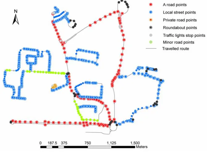
Figure 2: Trajectory data collected during data collection

A total of 983 point-based trajectory data was collected, 214 were on A roads, 400 on Local streets, 51 on Minor roads, 92 points on private roads with public access and 63 points on car parks (Table 1). Using the Ordnance Survey road class naming conventions, roundabout features are normally part of other road classes say A roads, Local streets or minor roads. But for our purpose we treat roundabout features and points collected at traffic lights stops as unique classes considering the fact that we are grouping the trajectory data based on geometry and topology information between successive points.

Table 1: composition of the GPS-based trajectory data within the different road

classes

Road feature GPS points

A road 214

Local street 400

Minor road 51

Private road public access 92

Car park 62

Roundabout 103

Traffic lights 61

Total 983

5.1. Data processing

The geographical distance between successive GPS points are calculated using the Haversine solution [19] as presented:

∆lat = lat2 – lat1 (1)

∆long = long2 – long1 (2)

a = sin2_{(∆lat/2) + cos(lat1) * cos(lat2) *}

sin2_{(∆long/2) (3)}

C = 2 * atan2 (√a, √(1-a)) (4)

D = R*C (5)

Where R = 6.371 Km; presuming a spherical earth with radius R, and that the locations of the two points in spherical coordinates. Given the distance and time, the speed between successive points is easily derived. The bearing from successive points to the previous was calculated using the rhumb line solution [20] presented below:

∆φ = ln [tan(lat2/2 + π/4)/tan(lat1/2 + π/4)] (6)

α = atan2(∆long, ∆φ) (7)

Where ln is the natural log and α is the bearing.

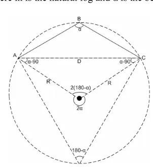
Figure 3: Derivation of horizontal curvature using three successive GPS points

The radius of horizontal curvature between three successive points (example shown in Figure 3) was calculated as presented.

Consider three points A, B and C as shown in Figure 3;

αhor = (bearing from B to A) – (bearing from B to C) (8)

Using circle properties that opposite angles in a cyclic quadrilateral add up to 180 and angle at the centre of a circle is double the size of the angle at the edge, we can calculate the radius of horizontal curvature of points A, B and C as: -

The radius of vertical curvature between three successive points using the elevation information was calculated as presented:

From Figure 4,

β1= tan-1_(dist

A-B/∆H1) (10)

Where distA-Bis the distance from point A to B, ∆H1 is the absolute height difference between points

A and B.

Figure 4: Derivation of vertical curvature using three successive GPS points

Consequently,

β2= tan-1_(dist

B-C/∆H2) (11)

Then,

αver = β1+ β2 (12)

Like in equations 9,

Radius of vertical curvature = (13)

A 1-minute (12 successive points) moving average was carried on each data variable to remove sharp bumps (peaks or dips) caused by periods when there is insufficient satellites for GPS to function.

5.2. Input Representation for SDNN

The input dataset used for the snap-drift neural network (SDNN) is composed of 5 variables represented by separate fields in the input vector. These are the speed between successive points, rate of acceleration between successive points, radius of horizontal and vertical curvature between three successive points and change in direction between successive points. Table 2 shows the values ranges of the 5 variables used.

Table 2: Value ranges of input patterns Road segment properties Range

Speed 0.5 - 43.8Mph

Rate of acceleration 0.0 – 4.10Mph/s Radius of horizontal curvature 6.2 – 193.7m Radius of vertical curvature 0.0 – 193.8m Change in travel direction 00 _{– 353}0

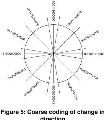
Coarse coding was used to represent the proportional differences between the changes in travel direction information since angle information span from 00 _to

3600_{. Thus the representation of angle 3}0 _{must be the}

same as that of say angle 3570_{; and similarly the}

representation 400 _{must be closer in input space to}

450 _{than that of say 55}0_{. Figure 5 shows the coarse}

coding implementation for the travel direction variable. 00001 1100 000 000001 110000 000000111000 0000₀₀₀₁ 1100 00₀₀ 00₀₀ 11₁₀ 000 0000 0011 1 1000000 0001 1 110000 000001 111000000000 0111₀₀₀₀ 0000 00₁₁ 10₀₀ 00₀₀ 0001 110 0000 0

Figure 5: Coarse coding of change in direction

As shown in Figure 5, 12 bit input coarse coding was used to represent the change in travel direction. For example 40 _{- 45}0 _{is represented as 000011100000}

and 460 _{– 86}0 _{is represented as 000001110000. In}

type might be repeatedly encountered while other are not encountered at all.

6. Results

Results are presented in Figure 6, 7 and 8(a-h) and in Table 3. Figure 6 shows the winning nodes and the road feature composition on each node. For instance, winning node 1 is made up of 35% A roads and local streets, 3% minor roads, 8% private roads with public access, 12% roundabout, and 4% traffic lights stops (Figure 6).

6.1. Sequences (Combinations) Grouping

On inspection of the dSDNN nodes, most of them have unique d-nodes sequences (dSeq) that in the majority of cases represent unique road related features (Figure 7). In this case winning node 1 is

separable, based on its d-node sequence, into 1-dSeqA for A roads and 1-dSeqL for Local streets and

1-dSeqR for roundabout features. Only the correctly

mapped (unique) d-node sequences are plotted in Figure 7. Based on the d-node output, the SDNN achieved overall grouping accuracy of 79.5%. Table 3 shows the grouping accuracy for each road class.

Table 3: Grouping accuracy of SDNN results Road Features Group accuracy

A road 97.2%

Local street 99.0% Private road 43.2% Minor road 29.4%

Roundabout 14.6% Traffic Lights stop 95.7%

Car park 82.0%

Figure 6: Plot of SDNN output showing the composition of different road feature in each winning node

6.3. SDNN trajectory grouping

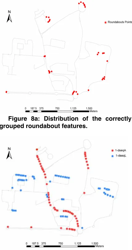
Figures 8(a-g) shows the spatial distribution of some of the SDNN grouped GPS-trajectory data. Only the correctly grouped points are shown. Figure 8a shows the distribution of those features that matched the Roundabout features. As can be seen in most of the point clusters, the distribution of the points does not quite make a “complete circle” feature like roundabout. Likely reason might be that the speed of travel while negotiating this feature was greater than the successive 5s time period adopted during the data collection. Another source of error could be due to the GPS carrier availability and precision which affects the position of collected points.

Figure 8a: Distribution of the correctly grouped roundabout features.

Figure 8b: Distribution of the unique d-nodes sequences from winning node 1.

Figure 8c: Distribution of the unique d-nodes sequences from winning node 2.

Figure 8d: Distribution of the unique d-nodes sequences from winning node 3.

Figure 8f: Distribution of the unique d-nodes sequences from winning node 7.

Figure 8g: Distribution of the unique d-nodes sequences from winning node 8.

Figure 8b shows the unique d-nodes sequences from winning node 1. This was made up of the A roads and Local street road types. The points in this category were more in the north-western directions. Similarly, Figure 8c shows those of winning node 2.

Figure 8d shows the unique d-nodes sequences from winning node 3. This was made up of the A roads, local streets and private road types. Also Figure 8e shows the distribution of points for the unique d-nodes sequences from winning node 6. The grouping is made up of input patterns corresponding to the A roads and local street.

Figure 8f shows the unique d-nodes sequences from winning node 7. This is made up of A roads and local streets. Also figure 8g shows the distribution of points for the unique d-nodes sequences from winning node 8. Input patterns from local street and A roads were grouped into this winning node. Majority of the patterns grouped in this node are those of local street road types. Only two input pattern from the A road types are grouped into this node.

6.4. Comparison with LVQ

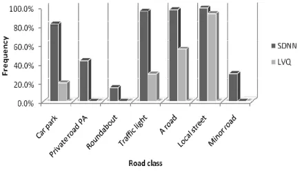
Figure 9 shows a comparison of the correct SDNN grouping with that of a typical LVQ neural network for each road class. For instance, 82% of car park input patterns are correctly classified by SDNN compared to 19.7% by LVQ. The SDNN achieved an overall class accuracy of 79.51%, compared to 51.78% for LVQ grouping. This result shows that the SDNN is able to recognise finer features of the road classes’ input patterns compared to a typical LVQ.

Figure 9: Plot showing comparison of correctly grouped between the SDNN and

LVQ neural network

Figure 10 shows the distribution of all correctly grouped points. Visual inspection of the distribution of the points shown in Figure 10 shows that the SDNN is able to group the trajectory data in such a way that it corresponds to different road feature classes. Most of the errors were largely due to confusion between private roads, minor roads and

traffic light stops. This is explained by the fact that the road inputs for the aforementioned classes are characterised by similar variables and in reality variables like speed regimes and acceleration on these road classes rarely differ. For instance, on most of these roads, cars were parked along the roads thereby causing a reduction in the drive speed (increase in collected GPS points). In addition the small number of inputs for these classes available for training compared to other classes (Table 1) could also affect the grouping accuracy of these classes. Errors in the roundabout features were mostly attributed to the travel speed and GPS precision during data collection.

7. Conclusions and future work

The result of the vehicle trajectory similarity grouping using SDNN offers a fast method of learning that preserves feature discovery and is capable of grouping moving object characteristics according to their local context information.

Consequently these groupings can inform whether the road feature travelled is new road feature that needs to be added to existing road database. Although using only GPS-related information as shown in this work has achieved grouping accuracy above 70%, another option still to be exploited is to incorporate neighbourhood information of GPS

have shown improved classification accuracy of about 93%.

8. Acknowledgements

The authors grateful acknowledge the Ordnance Survey for provision of MasterMap coverages. All road centreline data in Figures 8(a-g) and 10 are Crown copyright.

9. References

1. Zhang, C., Towards an operational system for

automated updating of road databases by integration of imagery and geodata. ISPRS Journal of Photogrammetry and Remote Sensing, 2004. 58(3-4): p. 166.

2. Wessel, B., Road Network Extraction from SAR

Imagery Supported by Context Information. In: Proceedings of ISPRS congress "Geoinformation Bridging Continents", Istanbul, International Archieves of Photogrammetry, Remote Sensing and Spatial Information Sciences, Volume 35, Part 3B, pp. 360 - 365, 2004.

3. Holzapfel, W., M. Sofsky, and U.

Neuschaefer-Rube, Road profile recognition for autonomous car navigation and Navstar GPS support.

Aerospace and Electronic Systems, IEEE Transactions on, 2003. 39(1): p. 2.

4. Zhang, Q. A Framework for Road Change

Detection and Map Updating. in International Archives of the Photogrammetry, Remote Sensing and Spatial Information Sciences, Vol. 35, Part B2, pp.720-734. 2004.

5. Klang, D., Automatic detection of changes in

road databases using satellite imagery.

International Archives of Photogrammetry and Remote Sensing, 1998. 32 (Part 4): p. 293-298. 6. Gerke, M., et al., Graph-supported verification

of road databases. ISPRS Journal of Photogrammetry and Remote Sensing, 2004. 58(3-4): p. 152.

7. Hwang, J.R., H.Y. Kang, and K.J. Li.

Spatio-temporal similarity analysis between trajectories on road networks. in Lecture Notes in Computer Science (including subseries Lecture Notes in Artificial Intelligence and Lecture Notes in Bioinformatics). 2005.

8. Ramaswamy, H. and K. Toyama, Project

Lachesis: Parsing and modeling location histories. In Third International Conference, GIScience. 2004: p106-124. Springer-Verlag.

9. Hornsby, K. and M.J. Egenhofer, Modeling

moving objects over multiple granularities.

Annals of Mathematics and Artificial Intelligence, 2002. 36(1-2): p. 177-194.

10. Yutaka, Y., A. Jun-ichi, and S. Tetsuji, Shape-Based Similarity Query for Trajectory of Mobile Objects. Mobile Data Management: 4th International Conference, MDM 2003 Melbourne, Australia, January 21-24, 2003. Proceedings, 2003: p. 63-77.

11. Liu, X. and H.A. Karimi, Location awareness

through trajectory prediction. Computers, Environment and Urban Systems, 2006. 30(6): p. 741-756.

12. Ekpenyong, F., A. Brimicombe, and D.

Palmer-Brown, Updating Road Network Databases:

Road Segment Grouping Using Snap-Drift Neural Network. Geographical Information Science Research Conference (GISRUK’07), 2007. 11-13th April 2007, Maynooth, Ireland. 13. Barsi, A., C. Heipke, and F. Willrich, Junction

Extraction by Artificial Neural Network System - JEANS. International Archives ofPhoto grammetry and Remote Sensing, Vol. 34, Part 3B, pp. 18-21, 2002.

14. Jwo, D.J. and C.C. Lai, Neural network-based

geometry classification for navigation satellite selection. Journal of Navigation, 2003. 56(2): p. 291.

15. Winter, M. and G. Taylor. Modular neural

networks for map-matched GPS positioning. in

IEEE Web Information Systems Engineering Workshops (WISEW'03) pp. 106-111, December 2003. 2003.

16. Jwo, D.J. and C.C. Lai, Neural network-based

GPS GDOP approximation and classification.

GPS Solutions, 2007. 11(1): p. 51-60.

17. Lee, S.W., D. Palmer-Brown, and C.M.

Roadknight, Performance-guided neural network for rapidly self-organising active network management. Neurocomputing, 2004. 61: p. 5.

18. Lee, S.W. and D. Palmer-Brown. Phrase

recognition using snap-drift learning algorithm. in The Internation Joint Conference on Neural Neural Networks (IJCNN' 2005). 2005. Montreal, Canada, 31st July - 4th August.

19. Sinnott, R.W., Virtues of the haversine. Sky and Telescope, 1984. 68(159).

20. Veness, C., Calculate distance and bearing

between two Latitude/Longitude points. at