Optimal Generalized Biased Estimator in Linear Regression Model

http://dx.doi.org/10.4236/ojs.2015.55042

Optimal Generalized Biased Estimator in

Linear Regression Model

Sivarajah Arumairajan

1,2

_{, Pushpakanthie Wijekoon}

3

1_{PostgraduateInstitute of Science, University of Peradeniya, Peradeniya, Sri Lanka}

2_{Department of Mathematics and Statistics, Faculty of Science, University of Jaffna, Jaffna, Sri Lanka} 3_{Department of Statistics & Computer Science, Faculty of Science, University of Peradeniya, Peradeniya, Sri} Lanka

Email: [email protected], [email protected]

Received 3 June 2015; accepted 2 August 2015; published 5 August 2015

Copyright © 2015 by authors and Scientific Research Publishing Inc.

This work is licensed under the Creative Commons Attribution-NonCommercial International License (CC- BY-NC).

http://creativecommons.org/licenses/by-nc/4.0/

Abstract

The paper introduces a new biased estimator namely Generalized Optimal Estimator (GOE) in a multiple linear regression when there exists multicollinearity among predictor variables. Sto-chastic properties of proposed estimator were derived, and the proposed estimator was compared with other existing biased estimators based on sample information in the the Scalar Mean Square Error (SMSE) criterion by using a Monte Carlo simulation study and two numerical illustrations.

Keywords

Multicollinearity, Biased Estimator, Generalized Optimal Estimator, Scalar Mean Square Error

1. Introduction

However, the researchers are still trying to find the best estimator by changing the matrix A compared to the already proposed estimators based on sample information. Instead of changing A, in this research we introduce a more efficient new biased estimator based on optimal choice of A.

The rest of the paper is organized as follows. The model specification and estimation is given in Section 2. In Section 3, we propose a biased estimator namely Generalized Optimal Estimator (GOE), and we obtain its sto-chastic properties. In Section 4 we compare the proposed estimator with some biased estimators in the Scalar Mean Square Error criterion by using a real data set and a Monte Carlo simulation. Finally some conclusion re-marks are given in Section 5.

2. Model Specification and Estimation

First we consider the multiple linear regression model

(

2

)

, ~N 0,

σ

= +

y X

β ε ε

I (1) where y is an n×1 observable random vector, X is an n p× known design matrix of rank p, β is a p×1 vector of unknown parameters and ε is an n×1 vector of disturbances.

The Ordinary Least Square Estimator of β and

σ

2 _{are given by} 1

ˆ₌ − _′ S X y

β (2)

and

(

) (

)

2

ˆ ˆ

ˆ

n p σ

′

− −

=

−

y Xβ y Xβ

(3)

respectively, where S=X X′ .

The Ridge Estimator (RE), Almost Unbiased Ridge Estimator (AURE), Liu Estimator (LE) and Almost Un-biased Liu Estimator (AULE) are some of the Un-biased estimators proposed to solve the multicollinearity problem which are based only on sample information. The estimators are given below:

RE: βˆ_RE

( )

k =Wβˆ where

(

1

)

1 k − −

= +

W I S for k≥0

LE: βˆ_LE

( )

d =F_dβˆ where F_d =

(

S+I

) (

−1 S+dI

)

for 0≤ ≤d 1

AURE: βˆ_AURE

( )

k =A_kβˆ where 2

(

)

2

k k k

−

 

=_ − + _

A I S I for k≥0 AULE: βˆ_AULE

( )

d =T_dβˆwhere T_d =_I− −

(

1 d

) (

2 S+I

)

−2_ for 0≤ ≤d 1

Since RE, LE, AURE and AULE are based on OLSE, [5] proposed a generalized form to represent these four estimators, the Generalized Unrestricted Estimator (GURE) which is given as

( )

ˆ ˆ

GURE =Ai

β β (4)

where A_{( )i} is a positive definite matrix and A_{( )i} stands for W, F_d, A_k and T_d . The bias vector, dispersion matrix and MSE matrix of

β

ˆ_GURE are given as

( )

ˆGURE =

(

( )i −

)

B β A I β (5)

( )

ˆGURE

σ

2 ( )i 1 ( )i − _′ =

D

β

A S A (6) and

( )

ˆGURE 2 ( )i 1 ( )i ( )i

(

( )i1

)

(

( )i1

)

( )i

MSE β =σ A S A− ′ +A I−A− ββ′ I−A− ′A′ (7)

respectively.

3. The Proposed Estimator

From (7) the following equation can be obtained by taking trace operator as

( )

ˆGURE 2

(

( )i 1 ( )i

)

(

( )i1

)

( ) ( )i i

(

( )i1

)

tr MSE_

β

_=

σ

tr A S A− ′ +

β

′ I−A− ′A A′ I−A−

β

(8)

By minimizing (8) with respect to A_{( )i} , the optimum A_{( )i} can be obtained.

( )

{

}

( ) ( ) ( )

(

)

( ) ( ) 1 2 ˆ

GURE _{i i}

i i i

tr MSE tr

σ −     ∂ _{ } ∂_ ′ _{ ∂ ′} = + ∂ ∂ ∂

A S A _B

A A A

β _{β β}

(9)

where B=

(

I−A_{( )}−_i1

)

′ ′A A_{( ) ( )i i}

(

I−A_{( )}−_i1

)

Now we can simplify the matrix B as

( )

(

)

( ) ( )

(

( )

)

( ) ( ) ( ) ( )

1 1

i i i i

i i i i

− ′ ′ −

= − −

′ ′

= − − +

B I A A A I A

A A A A I

Therefore

( ) ( ) ( ) ( )

( ) ( ) ( )

2

i i i i

i i i

′ = ′ ′ − ′ ′ − ′ + ′

′ ′ ′ ′

= − +

B A A A A

A A A

β β β β β β β β β β

β β β β β β (10)

Now we will use the following three results (see [6], p. 521, 522) to obtain the

(

( ) ( )

)

( ) 1 i i i tr −  _′  ∂   ∂ A S A

A and

( )i

′ ∂ ∂ B A β β .

(a) Let M and X be any two matrixes with proper order. Then

(

)

₍

₎

tr ′ ∂ ′ = + ∂ XMX

X M M

X

(b) If x is an n-vector, y is an m-vector, and C an n m× matrix, then

∂ _{′ = ′}

∂C x Cy xy

(c) Let x be a K vector, M a symmetric T T× matrix, and C a T×K matrix. Then 2

′ ′

∂ _{= ′}

∂ x C MCx

MCxx C

By applying (a) we can obtain

( ) ( )

(

)

( ) ( )

(

)

( )

1

1 1 1

2 i i i i i tr − − − −  _′  ∂_  = + = ∂ A S A

A S S A S

A (11)

Now we consider

( ) ( ) ( ) ( ) ( ) ( ) 2

i i i

i i i

  ′ ′ ′ ∂ ∂ ′ ∂ _{= −  }   ∂ ∂ _ ∂ _

A A A

B

A A A

β

β

β

β

β β

By using (b) and (c) we can obtain ( ) ( ) i i ′ ∂ ′ = ∂ A A

β

β

ββ

(13)

and ( ) ( ) ( ) ( ) 2 i i i i ′ ′ ∂ ′ = ∂ A A A A

β

β

ββ

(14)

respectively. Hence

( ) ( )

2 _i 2

i ′ ∂ _{′ ′} = − ∂ B A A

β β _{ββ ββ}

(15)

Substituting (11) and (15) to (9), we can derive that

( )

{

}

( ) ( ) ( )

2 1

ˆ

2 2 2

GURE i i i tr MSE σ −   ∂ _{ } ′ ′ = + −

∂A A S A

β

ββ ββ (16)

Equating (16) to a null matrix, we can obtain the optimal matrix A_{( )i} as

( )

(

)

1 2 1 i

σ

− − ′ ′ = + 

A

ββ

S

ββ

(17) Note that

(

σ

2 −1_{+ ′}

)

−1

S

ββ

exists since ₁+σ−2β β′_S ≠_{0 (see [6], p. 494).}

Now we are ready to propose a biased estimator namely Generalized Optimal Estimator (GOE) as ( ) ˆ

GOE = i

 _A

β

β

(18)

The bias vector, dispersion matrix, mean square error matrix and scalar mean square error of β_GOE can be obtained as

( )

GOE =

(

( )i −

)

B β A I β (19)

( )

GOE σ2 ( )i 1 ( )i − _′ =

  

D β A S A (20)

( )

GOE 2 ( )i 1 ( )i ( )i

(

( )i1

)

(

( )i1

)

( )i

MSE

β

 =

σ

A S A − ′ +A I−A−

ββ

′ I−A− ′A′ (21)

and

( )

GOE 2

(

( )i 1 ( )i

)

(

( )i1

)

( ) ( )i i

(

i1

)

SMSE

β

 =

σ

tr A S A −  +

β

′ I−A− ′A A ′ I−A−

β

(22)

respectively.

Note that since P=ββ′ is symmetric and P2=

ββ ββ

′ ′=

β ββ

2 ′=cP where 2 2 1 p i i c =

= β =

∑

β it can

be defined c 1 c

c

 

′ ′

= = _{ }=

 

P ββ ββ R. Then R′ =R and 2 =

R R. Therefore R is symmetric and idempotent matrix. Now we write the optimal matrix A_{( )i} as _{( )}

(

2 1

)

1

i c

σ

c

− −

= +



A R S R .

Now the bias vector, dispersion matrix, mean square error matrix and scalar mean square error of β_GOE can be rewritten as

( )

₂

(

₂

)

1

GOE σ σ c

−

= − +

 _{I RS}

( )

_{2 2}

(

_{2 1}

)

1 ₁

(

_{2 1}

)

1

GOE cσ σ c σ c

− −

− − −

= + +



D β R S R S S R R, (24)

( )

_{2 2}

(

_{2 1}

)

1 ₁

(

_{2 1}

)

1 ₄

(

₂

) (

1 ₂

)

1

GOE

MSE β =cσ R σ S− +cR − S− σ S− +cR − R+cσ σ I+cRS − R σ I+cRS − (25)

and

( )

_{2 2 2}

(

_{2 1}

)

1 ₁

(

_{2 1}

)

1 ₄

(

₂

)

2

GOE

SMSE β =cσ tr_σ R σ S− +cR − S− σ S− +cR − R_+σ β′ σ I+cRS − β (26)

respectively.

For practical situations we have to replace the unknown parameters

β

and

σ

2_{. For an estimated value for} β the OLSE, RE, LE, AURE or AULE can be used. For the estimated value for

σ

_ˆ2

we can use either (2) or replace βˆ in (2) by RE, LE, AURE or AULE accordingly. In the next section we will discuss the superiority of estimators when replacing each of these estimated values by using a simulation study, and then we use numerical examples for further illustration.

4. Numerical Illustration

4.1. Monte Carlo Simulation

To study the behavior of our proposed estimator, we perform the Monte Carlo Simulation study by considering different levels of multicollinearity. Following [7] we generate explanatory variables as follows:

(

₂

)

1 2

, 1

1 , 1, 2, , , 1, 2, , ,

ij ij i p

x = −γ z +γz + i=  n j=  p

where zij is an independent standard normal pseudo random number, and

γ

is specified so that the theoretical correlation between any two explanatory variables is given by γ2_{. A dependent variable is generated by using the} equation.

1 1 2 2 3 3 4 4 , 1, 2, , ,

i i i i i i

y =βx +β x +β x +β x +ε i=  n where ε_i is a normal pseudo random number with mean zero and variance 2

i

σ . [8] have noted that if the MSE is a function of

σ

2

and β , and if the explanatory variables are fixed, then subject to the constraint β β′ , the MSE is minimized when

β

is the normalized eigenvector corresponding to the largest eigenvalue of the X X′ matrix. In this study we choose the normalized eigenvector corresponding to the largest eigenvalue of X X′ as the coefficient vector

β

, n=50, p=4 and 2

1 i

σ = . Four different sets of correlations are considered by se-lecting the values as

γ

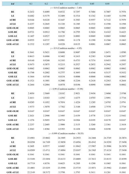
=0.8, 0.9, 0.99 and 0.999.

Table 1 can be obtained by using estimated SMSE values obtained by using equations (7) and (21) for different shrinkage parameter d or k values selected from the interval (0, 1). The SMSE of GOE-OLSE, GOE-RE, GOE-LE, GOE-AURE and GOE-AULE are obtained by substituting OLSE, RE, LE, AURE and AULE in equation (21) respectively instead of

β

and

σ

2_.

According to Table 1, we can say that the GOE-OLSE has the smallest scalar mean square error values with compared to RE, LE, AURE, AULE, GOE-RE, GOE-LE, GOE-AURE and GOE-AULE when γ = 0.8, 0.9, 0.99 and 0.999.

4.2. Numerical Example

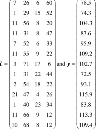
To further illustrate the behavior of our proposed estimator we consider two data sets. First we consider the data set on Portland cement originally due to [9]. This data set has since then been widely used by many researchers such as [10]-[13]. This data set came from an experimental investigation of the heat evolved during the setting and hardening of Portland cements of varied composition and the dependence of this heat on the percentages of four compounds in the clinkers from which the cement was produced. The four compounds considered by [9] are tri-calium aluminate: 3CaO∙Al2O3, tricalcium silicate: 3CaO∙SiO2, tetracalcium aluminaferrite: 4CaO∙Al2O3∙Fe2O3,

[image:6.595.81.534.106.716.2]

Table 1. Estimated SMSE values of the RE, LE, AURE, AULE, GOE-OLSE, GOE-RE, GOE-LE, GOE-AURE and GOE- AULE when γ = 0.8, 0.9, 0.99 and 0.999.

k/d 0.1 0.2 0.5 0.7 0.85 0.95 1

γ = 0.8 (Condition number = 3.40)

RE 0.2432 0.4089 0.6532 0.7297 0.7684 0.7887 0.7976

LE 0.6482 0.5179 0.2409 0.1514 0.1342 0.1465 0.1598

AURE 0.0166 0.0220 0.1647 0.3583 0.5557 0.7122 0.7979

AULE 0.4257 0.2845 0.1320 0.1385 0.1532 0.1590 0.1598

GOE-OLSE 0.0065 0.0065 0.0065 0.0065 0.0065 0.0065 0.0065

GOE-RE 0.0721 0.0912 0.1786 0.2795 0.3624 0.4163 0.4423

GOE-LE 0.1407 0.0527 0.0125 0.0083 0.0069 0.0065 0.0065

GOE-AURE 0.0555 0.0737 0.0981 0.1178 0.1390 0.1566 0.1663

GOE-AULE 0.1532 0.1207 0.0328 0.0135 0.0081 0.0067 0.0065

γ = 0.9 (Condition number = 4.95)

RE 0.3641 0.5621 0.8688 0.9687 1.0200 1.0471 1.0590

LE 0.8613 0.6906 0.3402 0.2415 0.2383 0.2698 0.2957

AURE 0.0140 0.0268 0.2183 0.4753 0.7374 0.9453 1.0593

AULE 0.5673 0.3875 0.2215 0.2527 0.2832 0.2942 0.2957

GOE-OLSE 0.0062 0.0062 0.0062 0.0062 0.0062 0.0062 0.0062

GOE-RE 0.1768 0.2002 0.2757 0.3693 0.4546 0.5137 0.5432

GOE-LE 0.1844 0.0740 0.0154 0.0088 0.0068 0.0062 0.0062

GOE-AURE 0.1521 0.1801 0.2080 0.2246 0.2418 0.2563 0.2644

GOE-AULE 0.2464 0.2004 0.0578 0.0196 0.0090 0.0065 0.0062

γ = 0.99 (Condition number = 15.99)

RE 2.4054 2.5669 2.8182 2.9021 2.9456 2.9686 2.9788

LE 2.4411 2.0183 1.4392 1.6275 2.0703 2.5091 2.7716

AURE 0.0285 0.1052 0.7054 1.4226 2.1285 2.6795 2.9791

AULE 1.9373 1.5078 1.7362 2.3188 2.6500 2.7578 2.7716

GOE-OLSE 0.0167 0.0167 0.0167 0.0167 0.0167 0.0167 0.0167

GOE-RE 2.2621 2.2908 2.3495 2.4159 2.4778 2.5219 2.5442

GOE-LE 1.1276 0.5055 0.0754 0.0304 0.0195 0.0170 0.0167

GOE-AURE 2.2257 2.2685 2.3000 2.3135 2.3260 2.3361 2.3418

GOE-AULE 2.2043 1.8384 0.5393 0.1438 0.0406 0.0190 0.0167

γ = 0.999 (Condition number = 50.55)

RE 23.6901 23.8842 24.1905 24.2933 24.3466 24.3749 24.3874

LE 20.0298 16.7109 12.9858 15.6956 20.4542 24.9250 27.5498

AURE 0.2405 0.9577 6.0485 11.9042 17.5907 21.9986 24.3876

AULE 16.8509 13.4711 17.0094 23.0107 26.3365 27.4124 27.5498

GOE-OLSE 0.1041 0.1041 0.1041 0.1041 0.1041 0.1041 0.1041

GOE-RE 23.5189 23.5494 23.6133 23.6889 23.7612 23.8133 23.8399

GOE-LE 10.7719 4.8376 0.6625 0.2305 0.1290 0.1065 0.1041

GOE-AURE 23.4801 23.5255 23.5590 23.5735 23.5871 23.5982 23.6045

We assemble our data set in the matrix form as follows:

7 26 6 60 78.5

1 29 15 52 74.3

11 56 8 20 104.3

11 31 8 47 87.6

7 52 6 33 95.9

11 55 9 22 109.2

and

3 71 17 6 102.7

1 31 22 44 72.5

2 54 18 22 93.1

21 47 4 26 115.9

1 40 23 34 83.8

11 66 9 12 113.3

10 68 8 12 109.4

  

 

 

 

 

 

 

 

 

 

 

=_{ } =

 

 

 

 

 

 

 

 

 

 

 

X y



 

 

 

 

 

 

 

 

 

 

 

 

 

 

 

 

 

 

 

 

 

 

.

For this particular data set, we obtain the following results: a) The eigen values of X X′ : 105, 810, 5965, 44663 b) The condition number = 20.58464

c) The OLSE of

β

is

β

ˆ

:

β

ˆ′ =

(

2.1930,1.1533, 0.7585, 0.4863

)

d) The OLSE of

σ

2

: 2

ˆ 5.8455

σ

= .

Table 2 can be obtained by using estimated SMSE values obtained by using Equations (7) and (21) for different shrinkage parameter d or k values selected from the interval (0, 1). The SMSE of GOE-OLSE, GOE-RE, GOE-LE, GOE-AURE and GOE-AULE are obtained by substituting OLSE, RE, LE, AURE and AULE in Equation (21) respectively instead of

β

and

σ

2

.

From Table 2 we can notice that the GOE-OLSE, GOE-RE, GOE-LE, GOE-AURE and GOE-AULE have the smallest scalar mean square error value with compared to RE, LE, AURE, AULE. Therefore we can suggest the GOE to estimate the regression coefficients. When k is large, GOE-OLSE has smallest SMSE than GOE-RE. When d is small, GOE-OLSE has smallest SMSE than GOE-LE.

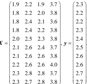
[image:7.595.233.396.103.319.2]

Now we consider the second data set on Total National Research and Development Expenditures as a Percent of Gross National product originally due to [14], and later considered by [15]-[17].

Table 2. Estimated SMSE values of RE, LE, AURE, AULE, GOE-OLSE, GOE-RE, GOE-LE, GOE-AURE and GOE- AULE the data set on Portland Cement.

k/d 0.1 0.2 0.5 0.7 0.85 0.95 1

RE 0.0637 0.0636 0.0633 0.0632 0.0631 0.0631 0.0630

LE 0.0631 0.0631 0.0633 0.0635 0.0636 0.0637 0.0638

AURE 0.0638 0.0638 0.0638 0.0639 0.0639 0.0640 0.0641

AULE 0.0638 0.6368 0.0638 0.0638 0.0638 0.0638 0.0638

GOE-OLSE 0.0003 0.0003 0.0003 0.0003 0.0003 0.0003 0.0003

GOE-RE 0.0003 0.0003 0.0004 0.0005 0.0006 0.0006 0.0006

GOE-LE 0.0006 0.0005 0.0004 0.0004 0.0003 0.0003 0.0003

GOE-AURE 0.0003 0.0003 0.0003 0.0003 0.0003 0.0003 0.0003

[image:7.595.90.540.548.723.2]

The data set is given below:

1.9 2.2 1.9 3.7 2.3

1.8 2.2 2.0 3.8 2.2

1.8 2.4 2.1 3.6 2.2

1.8 2.4 2.2 3.8 2.3

2.0 2.5 2.3 3.8 2.4 ,

2.1 2.6 2.4 3.7 2.5

2.1 2.6 2.6 3.8 2.6

2.2 2.6 2.6 4.0 2.6

2.3 2.8 2.8 3.7 2.7

2.3 2.7 2.8 3.8 2.7

  

  

  

  

  

  

  

  

= =

  

  

  

  

 

 

 

  

X y .

           

 

 

 



The four column of the 10 × 4 matrix X comprise the data on x₁, x₂, x₃ and x₄ respectively, and y is the predictor variable.

For this particular data set, we obtain the following results:

a) The eigen values of X X′ : 302.9626, 0.7283, 0.7283 and 0.00345 b) The condition number = 93.68

c) The OLSE of

β

is β βˆ: ˆ′ =

(

0.6455, 00896, 0.1436, 0.1526

)

d) The OLSE of σ2

: _ˆ2

0.0015

[image:8.595.238.389.97.243.2]

σ = .

Table 3 can also be obtained by using estimated SMSE values obtained by using Equations (7) and (21) for different shrinkage parameter d or k values selected from the interval (0, 1). The SMSE of GOE-OLSE, GOE-RE, GOE-LE, GOE-AURE and GOE-AULE are obtained by substituting OLSE, RE, LE, AURE and AULE in Equ-ation (21) respectively instead of

β

and

σ

2

.

From Table 3, we can say that our proposed estimator is superior to RE, LE, AURE and AULE, GOE-RE, GOE-LE, GOE-AURE and GOE-AULE.

5. Conclusions

[image:8.595.89.540.554.722.2]

In this paper we proposed a new biased estimator namely Generalized Optimal Estimator (GOE) in a multiple linear regression when there exists multicollinearity problem in the independent variables. The proposed estimator is superior to biased estimators which are based on sample information and takes the form βˆGURE =A_{( )}iβˆ. Based on Tables 1-3, it can be concluded that the proposed estimator has smallest scalar mean square error values com- pared with RE, LE, AURE and AULE. We can also suggest that GOE-OLSE is the best estimator with compared to GOE-RE, GOE-LE, GOE-AURE and GOE-AULE.

Table 3.Estimated SMSE values of RE, LE, AURE, AULE, GOE-OLSE, GOE-RE, GOE-LE, GOE-AURE and GOE-AULE the data set on total national research and development expenditures.

k/d 0.1 0.2 0.5 0.7 0.85 0.95 1

RE 0.1247 0.1664 0.2088 0.2202 0.226 0.2291 0.2304

LE 0.1881 0.1519 0.0797 0.0619 0.0645 0.0739 0.0808

AURE 0.0214 0.0155 0.0549 0.1096 0.1645 0.2077 0.2313

AULE 0.1362 0.086 0.0213 0.025 0.0453 0.0671 0.0808

GOE-OLSE 0.0000 0.0000 0.0000 0.0000 0.0000 0.0000 0.0000

GOE-RE 0.1169 0.163 0.2076 0.2194 0.2253 0.2284 0.2298

GOE-LE 0.186 0.1469 0.0573 0.0206 0.0052 0.0006 0.0000

GOE-AURE 0.0568 0.1093 0.1724 0.1899 0.1987 0.2033 0.2053

Acknowledgements

We thank the Postgraduate Institute of Science, University of Peradeniya, Sri Lanka for providing all facilities to do this research.

References

[1] Hoerl, E. and Kennard, W. (1970) Ridge Regression: Biased Estimation for Nonorthogonal Problems. Technometrics,

12, 55-67. http://dx.doi.org/10.1080/00401706.1970.10488634

[2] Singh. B., Chaubey. Y.P. and Dwivedi, T.D. (1986) An Almost Unbiased Ridge Estimator. Sankhya: The Indian Jour-nal of Statistics B, 48, 342-346.

[3] Liu, K. (1993) A New Class of Biased Estimate in Linear Regression. Communications in Statistics—Theory and Me-thods, 22, 393-402. http://dx.doi.org/10.1080/03610929308831027

[4] Akdeniz, F. and Kaçiranlar, S. (1995) On the Almost Unbiased Generalized Liu Estimator and Unbiased Estimation of the Bias and MSE. Communications in Statistics—Theory and Methods, 34, 1789-1797.

http://dx.doi.org/10.1080/03610929508831585

[5] Arumairajan, S. and Wijekoon, P. (2014) Generalized Preliminary Test Stochastic Restricted Estimator in the Linear regression Model. Communication in Statistics—Theory and Methods, In Press.

[6] Rao, C.R. and Touterburg, H. (1995) Linear Models, Least Squares and Alternatives. Springer Verlag. http://dx.doi.org/10.1007/978-1-4899-0024-1

[7] McDonald, G.C. and Galarneau, D.I. (1975) A Monte Carlo Evaluation of some Ridge-Type Estimators. Journal of American Statistical Association, 70, 407-416. http://dx.doi.org/10.1080/01621459.1975.10479882

[8] Newhouse, J.P. and Oman, S.D. (1971) An Evaluation of Ridge Estimators. Rand Report, No. R-716-Pr, 1-28.

[9] Woods, H., Steinour, H.H. and Starke, H.R. (1932) Effect of Composition of Portland Cement on Heat Evolved during Hardening. Industrial and Engineering Chemistry, 24, 1207-1214. http://dx.doi.org/10.1021/ie50275a002

[10] Kacıranlar, S., Sakallıoğlu, S., Akdeniz, F., Styan, G.P.H. and Werner, H.J. (1999) A New Biased Estimator in Linear Regression and a Detailed Analysis of the Widely Analyzed Dataset on Portland Cement. Sankhyā, Ser. B, 61, 443- 459.

[11] Liu, K. (2003) Using Liu-Type Estimator to Combat Collinearity. Communications in Statistics—Theory and Methods,

32, 1009-1020. http://dx.doi.org/10.1081/STA-120019959

[12] Yang, H. and Xu, J. (2007) An Alternative Stochastic Restricted Liu Estimator in Linear Regression. Statistical Papers,

50, 639-647. http://dx.doi.org/10.1007/s00362-007-0102-3

[13] Sakallıoğlu, S. and Kaçiranlar, S. (2008) A New Biased Estimator Based on Ridge Estimation. Statistical Papers, 49, 669-689. http://dx.doi.org/10.1007/s00362-006-0037-0

[14] Gruber, M.H.J (1998) Improving Efficiency by Shrinkage: The James-Stein and Ridge Regression Estimators. Dekker, Inc., New York.

[15] Akdeniz, F. and Erol, H. (2003) Mean Squared Error Matrix Comparisons of Some Biased Estimators in Linear Re-gression. Communication in Statistics—Theory and Methods, 32, 2389-2413.

http://dx.doi.org/10.1081/STA-120025385

[16] Li, Y. and Yang, H. (2011) Two Kinds of Restricted Modified Estimators in Linear Regression Model. Journal of Ap-plied Statistics, 38, 1447-1454. http://dx.doi.org/10.1080/02664763.2010.505951