Preferences and Increased Risk Aversion under a General Framework of Stochastic Dominance

Munich Personal RePEc Archive

Preferences and Increased Risk Aversion

under a General Framework of Stochastic

Dominance

Donald C., Rudow

7 June 2005

Online at

https://mpra.ub.uni-muenchen.de/41191/

Preferences and Increased Risk Aversion under a General Framework of Stochastic Dominance

by

Donald C. Rudow

JUNE 7, 2005

Abstract

This paper analyzes increased risk aversion in the presence of two risks. Necessary and sufficient

conditions for increased risk aversion across the domain of the foreground risk are found for changes in

both the foreground and background risks. Preferences that satisfy the necessary and sufficient conditions

are determined through a lower bound on their measure of prudence. These bounds are found through

second-degree spreads of a transformation of the background risk. The necessary and sufficient conditions

demonstrate that for all second degree spreads of this nature, absolute temperance plays a central role in

the necessary and sufficient conditions for increased risk aversion. The approach also demonstrates that

changes in risk aversion under the general framework of stochastic dominating spreads can be explained

by a weighted average of terms involving absolute prudence and absolute temperance. Once a general set

of necessary and sufficient conditions have been found it is shown that for preferences that are decreasing

absolute risk averse in the sense of Ross, increased risk aversion due to changes in the background risk

within this framework is equivalent to Ross risk vulnerability. The general conditions also find necessary

and sufficient conditions for preferences to be properly risk averse toward patent increases in risk.

INDEX WORDS: Stochastic dominance, increased risk aversion, background risk, transformations,

Introduction

The existence of a background risk has been seen to be of particular interest in the research on

risk behavior. Ross (1981) observed that the Arrow-Pratt measure of risk aversion is inadequate in the

sense that upon the introduction of a background risk a more risk averse agent may not behave in a more

risk averse manner whenever a foreground risk is present. Other research has explored the effects of

aversion to risk upon the introduction of a stochastically independent background risk for certain types of

risk preferences as defined in Pratt and Zeckhauser (1987), Kimball (1993), and Gollier and Pratt (1996).

Gollier and Pratt demonstrate how these previously defined classes of risk preferences are related by

identifying sufficient conditions for any agent possessing these qualities to react to the introduction of a

small, unfair, and independent background risk by becoming more risk averse to bearing a foreground

risk. Their notion of preferences possessing these qualities, known as risk vulnerability, captures this

common quality for all of these classes of risk preferences and is the widest set of preferences upon which

the introduction of background risk will generate more risk averse behavior. However, Gollier and Pratt

do not present a systematic method for obtaining the different risk measures that arise in these various

cases.

The introduction of background risk has garnered a relatively greater share of the spotlight than

has the more common situation of background risk already being present. Eeckhoudt et al. (1996) have

derived necessary and sufficient conditions on utility for increased risk aversion under stochastic

dominating shifts in the distribution of the background risk. Their method yields conditions for greater

risk aversion whenever an already present background risk undergoes an unfavorable change in its

distribution. They derive conditions for increased risk aversion for arbitrary first degree stochastically

dominated spreads and then for arbitrary mean preserving spreads. Their approach can be extended to

arbitrary second degree spreads and this is the approach taken here. In doing so, the author believes a

greater understanding of increased risk aversion can be achieved under the general framework of

stochastic dominating spreads by focusing on that by which first degree spreads and mean preserving

necessary and sufficient conditions for increased risk aversion is seen to exist under the general

framework of second degree stochastic dominating spreads. These conditions reveal the importance

temperance and prudence both play in explaining changes in risk aversion within the framework of

stochastic dominating spreads in risk. It will be shown that the measure of temperance relative to

prudence helps explain any change in risk aversion under the general framework of stochastic dominance.

Once these universal conditions are known, specific transformations of the background risk will

yield necessary and sufficient conditions for increased risk aversion for families of von

Neumann-Morgenstern utility functions identifiable by conditions involving their measure of prudence. Once the

model has been developed to account for the presence of both risks, necessary and sufficient conditions

for increased risk aversion will include a condition on compensated increases in a foreground risk as well

as some comparative statics related to increases in background risk. Necessary and sufficient conditions

for preferences to be properly risk averse toward a patent increase in risk are identified.

Literature Review

The notion of more risk averse is equivalent to higher risk premiums. Pratt (1964) has shown the

risk premium, π, to be a function of the distribution of a foreground risk, θ, and an endowment, ω.

Defining F to be the cumulative distribution of this risk with compact support Θ, the risk premium solves

for the equality, _u



 

  

dF  u



_dF

  

  ,F





. Agent A is said to be locally more risk averse at wealth level ω than agent B when A’s risk premium at ω is higher than B’s, i.e.



,





,



A B

F F

    . Pratt has also shown that an agent with a higher risk premium at a given level of

wealth has a higher Arrow-Pratt measure of absolute risk aversion at this level as well, defined as

 

_{ }"  '

: _uu

r    _ . Preferences are said to be decreasing absolute risk averse whenever lower levels of wealth

The Arrow-Pratt measure of absolute risk aversion can be unreliable as an indicator that the more

risk averse will behave in a more risk averse way when a second risk is introduced. An agent that faces a

foreground risk may have a risk premium that changes in a manner not consistent with his Arrow-Pratt

measure of risk aversion upon the introduction of a second risk. Ross (1981) has shown that despite one

agent being uniformly more risk averse than another in the sense of Arrow and Pratt, i.e.,

 

 

A B

r   a r   , it is still possible for agent A to have a lower risk premium than agent B due to an

introduction of a background risk. This can occur in a lottery setting whenever the background risk is

associated with a particular payoff such that the likelihood of it occurring is sufficiently small. Pratt

(1990) adds clarity to this counterintuitive result by arguing that such behavior becomes more likely for

any agent that is more risk averse than A due to the greater relative importance placed by these agents on

changes in less desirable outcomes; while the less risk averse place greater relative importance on

changes in more desirable outcomesi.

Ross goes further and demonstrates that certain, more restricted preferences do not present such a

difficulty. Given any level of wealth, ω, if there exists a scalar a such that _{ } 1 _{ } 2

1 2

"' " " '

u u

u a u

 

 

 

  for any

wealth levels ω1 and ω2 contained in a sufficiently small interval centered at ω, then the agent exhibits

decreasing absolute risk aversion in the sense of Ross which implies decreasing absolute risk aversion in

the Arrow-Pratt sense. Satisfaction of this local condition for a von Neumann-Morgenstern utility

function assures us that the agent will have a higher risk premium whenever their Arrow-Pratt measures

of risk aversion increase. An example of how such information is useful involves the relationship between

risk premiums and insurance premiums. A background risk is an uninsurable risk. In the presence of a

background risk, individuals at best acquire partial insurance for foreground risks. A higher risk premium

following the introduction of a background risk implies a higher willingness to pay for partial insurance

of a foreground risk in the presence of a background risk. Decreasing absolute risk aversion in the sense

Kihlstrom et al. (1981) confirmed Ross’s conclusion that the Arrow-Pratt measure of risk

aversion is unreliable as an indicator of risk averse behavior in general upon the introduction of

background risk, even if the two risks are statistically independent. Nonetheless, they go on to

demonstrate the usefulness of statistically independent risks in deriving comparative statics results and

proved that under this restriction, nonincreasing absolute risk aversion is preserved for expected utility,

i.e. _uu_'"_{ } __ _uu_{' }" _ _{E u}E u__'"_{    }    _{ } _{| ,}| ,_ _{E u}E u__'"_{  }  __||_

   

   with θ < 0. They also demonstrate that when the agent

is decreasing absolute risk averse in the sense of Ross, expected utility inherits this property as long as the

independence condition holds between the two random variables. Under the assumption of statistically

independent risks, they discover that higher risk premiums are associated with higher Arrow-Pratt

measures of risk aversion following the introduction of a statistically independent background risk as long

as preferences are nonincreasing absolute risk averse.

Absolute prudence has gained some prominence in the literature of the theory of risk. Kimball

(1990) describes prudence as ‘a propensity to forearm oneself in the face of uncertainty’. Unlike the

measure of absolute risk aversion, which measures the intensity by which an individual likes or dislikes

risk at a given level of wealth, prudence measures the sensitivity of a decision variable under conditions

of optimality. Quite often prudence is referred to as the precautionary motive, or an individual is said to

be prudent when the third derivative of the utility function is positive. It is well known that decreasing

absolute risk aversion implies an agent’s measure of absolute prudence is no less than his measure of

absolute risk aversion. Prudence proves to play a central role in identifying preferences that experience

increased risk aversion in this paper.

The behavioral condition on preferences that an unattractive lottery can never become more

attractive due to the presence of another independent, unattractive lottery accurately describes properly

risk averse preferences and was originally introduced by Pratt and Zeckhauser (1987). An agent who is

properly risk averse will have a higher risk premium upon the introduction of an independent risk at any

nonrandom and preferences are properly risk averse, this will be referred to as ‘fixed wealth proper’ risk

averse preferences. Utility functions that are properly risk averse are also decreasing absolute risk averse

in the Arrow and Pratt sense.

Kimball (1993) considered the set of independent aggravating risks. A risk is

loss-aggravating if the reduction in expected utility increases as wealth is reduced by a small amount once that

risk has been introduced. That is to say, ε is loss-aggravating for a decrease in wealth of size δ > 0 if



 



  



E u_   u     _u  u   . For an infinitesimally small reduction in wealth this is

equivalent in the limit to Eu'



 



u'

 

 . A statistically independent background risk will be loss aggravating for preferences that are standard risk averse when an undesirable risk is already present.

Kimball proves that necessary and sufficient conditions for preferences to be standard risk averse are that

absolute prudence, defined as p

 

 :_uu_""'_{ }  , and absolute risk aversion be decreasing in wealth. Standard risk averse preference are also properly risk averse.

Risk vulnerable preferences are the most general class of preferences that satisfy the attractive

quality of more risk averse preferences behaving in a more risk averse manner when a statistically

independent background risk is introduced. Gollier and Pratt (1996) define preferences as being risk

vulnerable when the introduction of any unfair background risk makes the agent behave in a more risk

averse manner. In the case of a small fair background risk, they provide an expression that approximates

the local relative change in the risk premium due to the introduction of the risk,

     

     

 

    _{ }  

    4 2 "

"' '

2

, ,

, 2

u Eu

u Eu

E p r

r

F F

F r E p r

  

  

  



  

     

 



 

  

   

  _{ }



 

where 





,F



is the risk premium that solves for the following equality in the presence of a

background risk with distribution H and compact support Ε;



    



 



,





 

u    dF  dH  u   dF   F dH 

         

A necessary and sufficient condition for risk vulnerability is that for every level of wealth both absolute

prudence and absolute temperance, defined as

 

 _{ } 

4

"'

: u_u

t   _ , are no less than absolute risk aversion.

Generally speaking, preferences are said to be locally risk vulnerable at ω if p

   

 r  and

   

t  r  . They note necessary and sufficient conditions for various classes of risk preferences that must hold for local risk vulnerability and discover that properly risk averse and standard risk averse

preferences are risk vulnerable.

Rothschild and Stiglitz (1970) provide a definition for an increase in risk as a mean preserving

spread of the risk. A distribution F parameterized by α1 is said to undergo a mean preserving spread

indexed by parameter α2 when the following conditions are satisfied:

 

2



1



0,

; ;

0,

F t F t dt

 



 

     

 _  _

  _{ }



(1.1)

Where the ‘underbar’ and ‘overbar’ notation denotes the minimum and maximum elements of the

compact support of F (Θ) respectively. This is a special case of second degree stochastic dominance, and

throughout the paper this condition, commonly referred to as a Rothschild-Stiglitz increase in risk, will be

expressed as the partial ordering,F



 ; ₁



MP F



 ; ₂



. An important result of their paper is that any risk

averse agent when given the choice of the lotteries indexed by α1 and α2 will reject the lottery indexed by

α2 whenever (1.1) holds. That is, for any concave utility function, u(θ), _u

  

 dF  ; 1



_u

  

 dF  ; 2



whenever the conditions given in (1.1) are satisfied.

Eeckhoudt et al. (1996) utilize the notion of first degree stochastically dominated and mean

preserving increases in background risk to provide a framework for analyzing an agent’s behavior under

such changes in an already present background risk. They derive necessary and sufficient conditions for

increased risk aversion within this setting that are specific to the nature of the stochastic dominating shift

of the background risk that occurs. If it is a first degree stochastic dominating shift over the compact

 

2



1



0,

; ;

0,

d H t H t

 



 

     

 _ _

 _{  }



then decreasing absolute risk aversion in the sense of Ross is necessary and sufficient for increased risk

aversion. On the other hand, if the background risk undergoes a mean preserving spread in the

background risk then another boundedness condition, t



 



 

  

r  



, is necessary and sufficient for increased risk aversion. They conclude that both conditions must be satisfied if any second

degree spread in background risk is to cause increased risk aversion. One result of this paper confirms

their result but also proves that for any stochastic dominating spreads of a second degree nature that is not

a first degree spread, their conditions are indeed sufficient but not necessary for increased risk aversion.

An alternative definition of increases in risk involves the use of utility distributions. Diamond and

Stiglitz (1974) consider mean preserving spreads in the distribution of utility via change of variable

techniques. They note that if marginal utility is nonzero, change of variable techniques yield a set of

conditions that hold under mean preserving spreads in utility. Thus, if F is the utility distribution

function indexed by the distribution of F



 ;



, and α2 indexes a mean preserving spread in F, then



; 1



MP



; 2



F U  F U  where U u

 

 , and it follows that

 



 

2





 

1



 



2





1



0,

, ; ; ;

0,

u t F u t F u t dt u t F F dt

 

 

 



     

     

 _  _  _  _

    _{ }





A mean preserving utility spread is conveniently viewed as a compensated increase in risk. Such a spread

in risk for an individual is not preferred by anyone more risk averse as indicated by a higher Arrow-Pratt

measure of absolute risk aversion.

Transformations of random variables have been utilized to alter the mean and variance of risk

within an optimization problem (Sandmo (1971)) and cause a Rothschild-Stiglitz increase in risk (Meyer

and Ormiston (1989)). A deterministic transformation of a random variable is nondecreasing in the

random variable. Such a transformation preserves the ranking of preferences in a stochastic environment.

   

1 2 1 2

k  k     . Meyer ((1977) and (1989)) has also analyzed such transformations under a

stochastic dominance framework in an effort to rank deterministic transformations of a random variable.

Meyer describes stochastic dominance with respect to a function as:







  

 









 

 

 



"



2 1 2 1 '

; ; ; ; 0 _kk ,

F t F t dk u d F F u

 _



          

 

             

   





Hence, any agent with absolute risk aversion greater than or equal to _kk_{' }" _ will choose the lottery indexed by α1 over that indexed by α2 when forced to choose between these two lotteries. Meyer’s research has

successfully generalized the notion of stochastic dominance. The results that follow differ from that of

Meyer in several respects. First, all families of utility functions with prudence measures that are pointwise

bounded from below by a similar looking ratio for the transformation of the background risk space will

experience increased risk aversion whenever the distribution undergoes a second degree spread in the

transformed background risk. Secondly, all preferences with prudence measures that exceed the

aforementioned bound will experience an increase in their expected marginal utilities under the

deterioration in background risk. Finally, all stochastic dominating spreads will be occurring for

transformations of background risks rather than background risks directly.

Increased Aversion to Risk

Introductions of risk, often a relevant part of the definition of classes of risk preferences as in the

case of Pratt and Zeckhauser (1987), Kimball (1993), and Gollier and Pratt (1996), may be considered to

be nothing more than an increase in the variance of an ‘improper’ distribution. An improper distribution

for any risk will be one in which there is no variance, i.e. all the probability mass occurs at some

particular value. When this is the case, with H the distribution function for the background risk, parameter

β1 will be the parameter that represents an improper distribution for the background risk. Either a first or

second degree stochastically dominated increase in background risk indexed by ‘j’, may occur when a

It will be convenient to work with an indirect utility function in what immediately

follows. Following convention, let v



 ; i



_u

 

 , dH



 ; i



be the indirect utility function indexed by

parameter βi. Indirect utility is strictly monotonic in θ, indicating v



; i



V i



   can be inverted to apply

the change of variable technique. For a nontrivial second degree stochastic dominating spread in indirect

utility, _Vi_{, the appropriate conditions are}









 

 







 



min

0,

; ; ; ; ;

0, some

i V

w h w h i

v F t F t dt F s F s v s ds

 _

 



    

 

   

    _  _{ }

  _{ }





(2.1)

Any distribution by definition is a second degree spread of itself and is sometimes referred to as a null

spread. Such spreads are of no interest in this paper. Nonetheless, it is possible for null spreads to be the

only types of spreads that satisfy certain conditions. For any second degree spread it will be assumed that

there is some θ for which (2.1) is a strict inequality, thereby ruling out null spreads.

Keenan and Snow (2003) have shown that when background risk is initially absent, β = β1, any

compensated increase in risk satisfying (2.1), with equality for θ equaling the maximum value of θ, that is

accompanied by the introduction of a small, fair, background risk reduces indirect utility if and only if the

introduction of the background risk causes the agent to be more risk averse in the sense of Arrow and

Pratt. Recognizing that a compensated increase in risk is specific to the individual’s preferences, this

result can be extended to include cases where the background risk is already present by making the

compensated increase in risk specific to the agent’s preferences given the presence of background risk.

The lemma below establishes this result. The proof makes use of the fact that any monotonically

increasing, concave utility function will be worse off under the distribution that is stochastically

dominated than it is under the distribution that stochastically dominates, as shown by Hadar and Russell

(1969).

Much of the analytical work that follows involves conditions that hold at the max or min of the

compact support for the cumulative distribution functions. These values will be recognized by the

Lemma 1: Let Ε be the support of H(ε;β), Θ be the support of F(θ;α) with background risk ε, and

foreground risk θ, independent random variables with c.d.f.s F and H respectively, where αw indexes a

compensated increase in risk for _Vi _{as in (2.1) with equality when}   _{. Define}





 

  " ; ' ;

; : i

i v

i _v

R     _{ }  .

For any utility function such that uθ > 0 and uθθ≤ 0:



; j





; w





; h



0

v   d F   F  

   

 for any αw satisfying (2.1) that is not a null spread with equality

holding when   if and only if R



 ; j



R



 ; i



for all .

Proof:













 

 



 







 

 



 







 

 



 







' ; ' , ' ; ' ; ' ; ' ; ; ; ; ' ; ; ; ' ; ; ; ' ; ; ; j i j j i i

j w h

v

i w h

v

v v

i w h i w h

v v

v d F F

v F F d

v s F s F s dsd v s F s F s ds

                                                    _  _   _{   }  _{  }  _  _  _  











Under a mean preserving spread of indirect utility, _Vi, indexed by the change in parameter from α

h to αw

the equality reduces to:













' ;

 

_{ }



 







' ;

; ; ; j ' ; ; ;

i v

j w h _v i w h

v d F F _   _v s F s F s dsd

                     _{ }      _{ }  







(2.2)

Notice that ' ;_{' ;}

 

_ j_ ' ;_{' ;}

 

_ j_





;





;





i i

v v

i j

v v R R

   

        



   . Hence the sign of the right hand side of (2.2) will be

determined by the difference in risk aversion due to a change in the parameter of the distribution

involving the background risk. Thus, when R



 ; j



R



 ; i



 it follows that



; j





; w





; h



0

v   d F   F  

   

 for any αw that indexes a change in the distribution of the

foreground risk satisfying (2.1). This proves sufficiency.

For necessity, I will prove the contra positive. Suppose that R



 ; j



R



 ; i



for some  ˆ .



; j





; i



R a  R a  for any aA. Then _v



 ; j



d F



 ; w



F



 ; h



0 for the following cumulative distribution function:

















, ; ; ; , ; i w h i

P V v A F V

F V V v A

            

Where P satisfies _{ }

















inf ;

0 ;

;

0, sup ;

i i V h v A i

V v A P F t dt

V v A

              _{ } 

 with a strict inequality over some subset

of v A



;i



and is known to exist by the integrand being continuous in P and

















 ; i inf ; i ; h ; h 0  ; i



sup





; i





; h





; h



v A F v A  F t dt  v A F v A  F t dt

 

This distribution possesses the quality of being stochastically dominated in a second degree sense and

yields the following terms after a change of variable, integrating over Θ rather than v



;i



.









   

_

_

_

_

min ; inf 0, ; ; ; ; , i V w h v i h A A F t F t dt

v s P F s ds A

                _{ }   _{   }    





Under this particular second degree spread in risk,

 

 



 







' ; ' ; 0, ' ; ; ; 0, j i v

i w h

v

A

v s F s F s ds

A   _                 _{  }    _{   }  





with a strict equality holding over some subset of A. Therefore,



; j





; w





; h



0

v   d F   F  

   



Q.E.D.

The change in parameter from βi to βj represents a shift in the distribution of the background risk

that causes the agent to be more risk averse. This increased aversion to risk is sufficient for the

compensated increase in risk for preferences _Vito be unattractive for preferences j

V indicated by the

decrease in the latter’s well-being. Any compensated increase in risk with background risk present that is

greater aversion to risk for all θ and a lower level of well being under the latter background risk. That is to

say, an unfavorable change in the distribution of the background risk also increases the agent’s aversion

to risk over the domain of the foreground risk (F). Observe at this point the distributions that both the βi

and βj parameters index bear no specific relation to each other.

Lemma 1 involves a special case of stochastic dominance with respect to a function as described

by Meyer (1977), modified only by the addition of background risk. That is, F



 ; _h



stochastically

dominates F



 ; _w



with respect to v



 ; _i



. This is Meyer’s necessary and sufficient condition for any

utility function with absolute risk aversion greater than R



 ; _i



that weakly prefers the distribution for

the foreground risk that dominates. Lemma 1 indicates that there exists indirect utility functions that

belong to this family, with the unique interpretation that all of these indirect utility functions will reject

the compensated increase in risk ‘constructed’ under the initial distribution for the background risk

indexed by βi. If this is true for all θ then any one of these other utility functions will not prefer the

compensated increase in risk for v



 ; _i



under the stochastically dominated distribution indexed by αw.

Thus the family of utility functions implied by greater aversion to risk in lemma 1 includes not only

indirect utility functions given by various second degree spreads of the background risk; but other indirect

utility functions as well including distributions of transformations of the background risk all of whom

share the common property of higher measures of absolute risk aversion for all θ. This aspect of the

lemma will be useful in understanding the results acquired in this paper as we examine stochastic

dominating spreads of functions of the background risk.

Transformed Background Risk and Prudence

Eeckhoudt et al. (1996) note that increased variance in the background risk can encompass more

complicated changes in the distribution than the analytically common case of adding another independent

risk. In the spirit of this particular observation, one goal of this paper is to treat a broad spectrum of

background risk domain (the domain of H). In doing so, second degree stochastic dominating spreads

encompass a richer set of distributions. An example of a stochastically dominated spread of a

transformation of risk has already been considered in (2.1) which involved a mean preserving spread of

the transformed foreground risk given by the mapping _vi: _Vi_{. The stochastic dominating}

relationship of interest in this case involved one existing over the transformed foreground risk. Generally

speaking, what I refer to as a transformed risk is the transformation of the compact support for a

distribution or the domain of the distribution. The transformed background risk will be given by the

transformation function :  , where Ε is the domain of the background risk. The purpose of this

type of transformation differs from that of deterministic transformations which seem to be most useful as

a means of altering a random variable under optimal choice problems.

The transformed background risk generalizes the notion of stochastic dominating spreads in a

simple manner. All spreads will be of the transformed background risk. To fix notation, denote the

cumulative distribution functions for the transformed background risk as H . Let  be a function of the

transformed background risk. Sticking with the tilde notation to emphasize what background risk is

relevant, the indirect utility function is seen to be



; i





 





, i



v   _u    dH   (3.1)

Changes in the parameter β index changes in the distribution of. Stochastic dominance of degree one or

two will be indexed by the partial ordering relation n.The relation conveys the idea that one distribution

stochastically dominates the other by degree ‘n’ where n equals 1 or 2. For a Rothschild-Stiglitz increase

in risk, the partial ordering is given by MP.

Increased risk aversion involving the transformed background risk is seen to be equivalent to the

following expression after a little algebraic manipulation1:





















" ; j " ; i ; i ' ; j ' ; i

v   v   R  v   v   

   _  _ (3.2)

1 _{Multipl y}



_;





_;



j i

R   R   by ' ;

 

_{" ;} j_

i v

v

   

To determine what conditions are associated with increased risk aversion culminating from arbitrary

second degree spreads of the transformed background risk we will initially focus on the basic idea that the

right hand side of (3.2) is of uniform sign. Doing so simplifies the task of signing two functions of interest

that are central to the results of this analysis. Fundamentally, nonnegativity of the right hand side for an

arbitrary second degree spread implies nonnegativity of the left hand side under the same conditions.

Whenever the right hand side of (3.2) is positive for arbitrary second degree spreads of  the sign of

 

'

  offers a sensible interpretation of the function  

 

within the framework of deterministic

transformations described by Meyer and Ormiston (1989). Analysis of the less restrictive condition that

the right hand side of (3.2) be nonnegative is simplified by the results obtained from the more restrictive

case. These results are central to all other results that follow. Given this, our first task is to find necessary

and sufficient conditions for









' ; j ' ; i ( )0 j

v   v      , where H



 ; i



2 H



 ; j



(3.3)

There are necessary and sufficient conditions for either sign in (3.3). I will proceed to informally

discuss the necessary and sufficient conditions that exist for the case of positive differences. It turns out

that the conditions concerning a decrease in indirect marginal utility will not be of interest in this paper

due to an issue discussed in Meyer and Ormiston. If utility is affected by the risk through a function such

that the function is nonincreasing in the domain of the risk, i.e.  '

 

0, then the ranking of lotteries

most likely will not be preserved. While conditions do exist for either sign and both will be given below,

it turns out that positive differences for (3.3) is the economically relevant one.

There are several observations to be made concerning subsets of the transformed background risk

for which the necessary condition for the difference in (3.3) being positive does not hold and it will be

seen that it is always possible to construct a second degree spread such that the difference in (3.3) is not

positive whenever one of the necessary conditions do not hold. This is a basic ‘not B implies not A’

those of a first degree nature as well as those of a mean preserving nature. Graphs of these various types

of second degree spreads will be considered prior to the formal proof. The function :  

 

is assumed to be twice differentiable. The necessary conditions for the difference in (3.3) to be positive are

 

 2



 



"

' 0

p  

    

 

 

   for almost all φ (3.4)

and

 

' 0

   _{for almost all φ} (3.5)

Considering the claim (3.5) initially, suppose   '

 

0 over some set denoted as t t

B B where

 





: : ' 0

B      and any Bt is connected. The closure of B, denoted as B consists of all the

elements of B and the limit points of B2. A first degree stochastic worsening in the distribution of the risk

 includes one in which the deterioration in the distribution involves leftward shifts of probability mass

occurring only over the closure of B, i.e. H



 ; j



H



 ; i



  B and H



 ; j



H



 ; i



  B.

Such a relationship can be generated from the distribution H



 ; i



by taking all of the probability

density implicitly assigned by the distribution over the closure of each of the sets Bt and assigning it all to

infBt. Calling the distribution that is the result of these new assignments in probability mass H



 ; j



,

this is the distribution generated from H



 ; i



that causes the condition











 



 









' ; j ' ; i _B " ' ; j ; i 0

v   v     u      _H   H   _d

given the defined set B. If the set B is a single point, then it has no effect on the integral, therefore, only

subsets of the transformed background risk that have some measurability are of issue. An example of a set

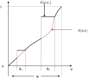
B is seen in Figure 1 below.

Given the infinite number of first degree stochastic worsening shifts in the distribution, it will

always be feasible to find a distribution such that the densities for both distributions differ only over

[image:18.612.103.410.117.389.2]

Figure 1

subspaces for which (3.5) is violated causing the marginal indirect utility differences to have the

undesired sign. Therefore, this must be a necessary condition for a positive value to exist in (3.3).

Now suppose _{ } 2



 



"

' p 0

 

    

 

     over some set t t

D D , where D is defined as

 

 2



 



" '

: : 0

D   p

 

   

 

 

 

_     _

  and any subset Dt is a connected set. Observe that the function

 

;

H s ds



 

 is convex and continuous although there may be a countable number of points in which it is

not differentiable. A second degree stochastically dominated spread in the distribution of  includes one

in which densities differ over the closure of the set D, but remain identical over the remaining space.

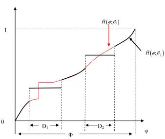
Assume the graph of Figure 2 represents a second degree stochastic deterioration in the distribution

φ

1

B

1

B

2



; i



H  

H(φ;β

)



; j



H  

H(φ;β

)

0

caused by taking the probability mass assigned by H



 ; i



over any Dt and assigning some of it to the

[image:19.612.101.439.188.474.2]

infimum of Dt and the rest of it to the supremum of Dt.

Figure 2

Assume that the relationship between the integrated cumulative distribution functions in Figure 2

satisfies the following conditions:

 





inf

0, and strictly so for some

; ;

0, sup i

i i

j i

D

i

D D

H s H s ds

D

 _{ }  



   



 _  _

  _{ }



It can be seen that H



 ; j



is a mean preserving spread of the risk given by the distribution H



 ; i



.

There is an increase in risk that occurs due to reassigning density over the subset D such that the

integrated difference of the two distributions is positive. The graph of these two integrated cumulative

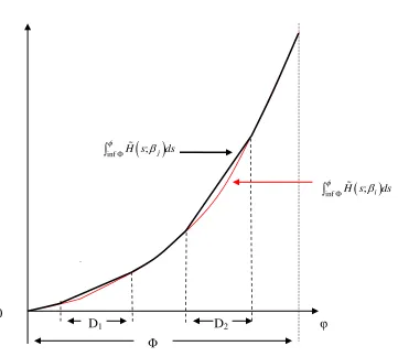
distribution functions may look something like Figure 3.

0

Φ

D

1

D

2

1

φ



; i



H  

H(φ;β

)



; j



H  

[image:20.612.107.468.91.415.2]

Figure 3

The cumulative distribution function derived from the original distribution, by redistributing the

density assigned under the original distribution across any of the subspaces Dt to that subspace’s infimum

and supremum, possesses the following qualities:

 





























1 1 2 2

1 1

2 2

; , ,inf sup ,inf sup ,

; sup ; int

sup ; int

i

j i

i

H D D D D

H s ds H D D

H D D



 

    

  

  



 _{   }

 

  



  



Generally speaking, the derivative of the integrated cumulative distribution function given by

parameter βj defines a cumulative distribution function for all but a countable number of points of Φ (a

finite number in this example). The densities between the two distributions differ only over the subspace

in which absolute prudence is sufficiently small enough to violate one of the proposed necessary

conditions.

0

Φ

D

1

D

2

φ

 

inf H s; j ds

 _









inf H s; i ds

 _



Over the subsets of the transformed background risk of which the two distributions are equal in

value, i.e. [ ,inf D1) [sup D1,infD2) [sup D2, ] , the difference between the integrated distributions seen

in Figure 2 is constant. In fact, the difference in the integrated distributions over the subset excluding the

set D is not only constant but is zero as well due to the differences in the integrated distributions being

zero for any  supDt. Knowing these properties, it can be seen that:











 



 

 

 2



 



 





2 "

'

' ; j ' ; i _D " ' ; j ; i 0

v v u   p _ H s H s dsd

 

              

 

 

 

 _{  }

 

   _{ }     _  _ 

 

 





Given this, a necessary condition must be that given in (3.4)   \D3 and the set D has measure zero4 whenever the difference in (3.3) is positive.

Unambigous statements concerning increases in an agent’s indirect marginal utility under any

mean preserving spread of an initial risk can be made about preferences based on their measure of

absolute prudence. The first degree condition restricts how the function of the transformed background

risk must enter the utility function for similarly unambiguous statements. Thus, satisfaction of both (3.4)

and (3.5) together are necessary for unambiguous changes in the marginal indirect utility functions due to

any type of second degree spread in the transformed background risk. What is immediately apparent is

that the function



may be viewed as a deterministic transformation. In fact, once the formal proof of this

is completed the function



will be treated as a special type of deterministic transformation.

Second degree stochastic deteriorations are obviously not all mean preserving spreads or first

degree spreads of. Yet it happens to be the case that the set of necessary and sufficient conditions are

given by these two specific forms of second degree spreads in risk. For a second degree spread in risk that

is neither mean preserving nor a first degree spread, consider a spread in risk occurring across the space

3_{Generally, the notation ‘X\Y’ refers to the set of all X that are not elements of Y.}

4_{It is assumed that Φ is subset in a space with Lebesgue measure. D  has Lebesgue measure zero whenever D}

is countable. Basic measure theory useful for economists can be found in Kirman (1981), although it is only useful if

you are familiar with measure theory. For our purposes, a set D has measure zero if for every  0there is a closed

cover of D,



G G1, 2,...



such that

 

i

i

G  

D1 (see Figure 2). Assuming it is not a mean preserving spread, a graph of the integrated cumulative

distribution functions will have slopes for both integrated cumulative distribution functions that are

identical everywhere except over the space D1. Some of the density assigned by H



 ; i



to D1 has been

shifted to the infimum of D1 while the remaining portion of the density has been assigned to its

supremum, generating a second degree spread in risk given by the distribution,









1

1

; ,

;

,

i j

H D

H

P D

    



 

  

 

For all D1 the slope of infD₁H s

 

; j ds

 _

[image:22.612.116.454.334.614.2]

 equals P. This is seen in Figure 4 below.

Figure 4

This particular relationship indicates that the sign of the difference in the integrated cumulative

distribution functions is determined entirely by the interval, infD1,. Given the assumption that for any

dDthere exists a G 



G G, ,...



such that dG . See Spivak (1965) for an informal elementary treatment of

0

Φ

φ

 

inf H s; j ds

 _









inf H s; i ds

 _





1

D

 the difference between the distributions is zero, the difference in the integrated cumulative

distribution functions is equivalent to:











 



 

 

 



 







 





 

 

 



 







 





 









2

1 1

2

1 1

2 "

inf '

2 "

sup _'

' ; ' ; " ' ;

" ' ;

- " ' ; ;

j i _{D D} i

i

D D

j i

v v u p P H s dsd

u p d P H d

u H H

  

 

  

 

             

           

        

 

 

 

 

 

  _{ }

 

   _{  }   _{ }  _

 

 

 

  _{ }

 

  _{  }   _{ }  _

 

 

 

 _  _









d





The first term on the right hand side of the equality is strictly nonpositive by assumption. The

sign of the second term is unknown while the sign of the third term is positive. Recognizing the fact that



; i



P H  

  

 

 is continuous in P, this factor can be made arbitrarily small while preserving the second

degree stochastic relationship between the two distributions. As





1 ; i

DPH s  

 approaches zero from

an initially positive value due to decreases in the value of P, the first term does not get smaller, i.e. its

magnitude does not get larger. This is due to the fact that over this subset, (3.4) is assumed to not be true.

In fact, a maximum value for the first term can be found. If this maximum value is negative, then the

difference in (3.3) will be negative for some second degree spread in risk regardless of the sign of the

derivative of the function



. A similar shift in the density over the subspace D2 can be performed as well,

but such a pursuit will turn out to be redundant and all that is needed is to find a distribution that causes









' ; j ' ; i 0

v   v    , which has been achieved.

The preceding discussion outlining the ‘not B implies not A argument’ provides the proper

framework to prove the necessary and sufficient conditions for the difference in (3.3) to be positive. For

the difference to be negative similar arguments can be made for the conditions given in lemma 2. The

proof will focus on first degree spreads and general second degree spreads in risk.

Lemma 2:Let :   with Ε compact, u’ > 0, and u” < 0. Let  C2

 

 be twice

continuously differentiable and H



 ; j



be an element of the set of all distributions for the transformed

background risk that satisfies

 

;



;



0

0 for some

j i

H s H s ds

           _  _   _{ }



Then: v'



 ; j



v'



 ; i



 ( )0 for any βj if and only if,

(i):   '

 

0 for almost all  (  '

 

0for almost all  )

(ii):



 



 

 2

"

'

p  

 

  

 

 

  for almost all  (



 



 

 2

"

'

p  

 

  

 

 

  for almost all .)

Proof: I will only prove the case for an increase in marginal indirect utility, seeing as the case of a

decrease follows similar arguments. Necessity is proven first. Suppose for all   B it is true that

 

' 0

   with B a set of nonzero measure. If this is true, then there is a distribution indexed by βj that

has a first degree stochastic relationship with βi such that v'



 ; j



v'



 ; i



0 where βj parameterizes

the distribution derived from H



 ; i



by shifting all the density over any subset of B to its infimum:

















sup ; , :

; , ,inf

t i t

t j

i t

H B B B

H

H B B t

                

This particular distribution has the partial ordering relationship H



 ; i



1 H



 ; j



with









' ; j ' ; i 0

v   v    .

Having established the necessary condition (i)suppose that  

 2



 



"

'

: : 0

D   p

              _     _    

has nonzero measure. If this is true, then let









1 1

inf

: P : D P H s; i ds 0 D

 _{   }

  _{ }  _   

P ,where D1 is a

measurable subset of D. For any PP there exists









1

inf

arg max D P H s; i ds P:



 

   

 

 





 

 

 2



 



₁





2 "

inf '

" ' _D ; i

u   p  P H s ds

                   _{ }    _{ }     _  _    



is nonincreasing in P for any  D1. Consequently,

 





 

_{ } 2



 







1 1

2 "

inf '

" ' ; i

Du p D P H s dsd

                       _{ }    _{  }   _{ }  _    





is nonpositive and nonincreasing in P as well. Define the maximum possible value for this integral over

1

D as

 



 



 

 

 2



 











1 1

2 "

inf '

: _D " ' _D min : ; i

M P u   p  P P H s dsd

                    _{ }     _{ }     _   _    





P .

Hence,

 





 

 

 2



 







 

1 1

2 "

inf '

" ' ; i 0

Du p D P H s dsd M P P

                       _{ }    _{  }   _{ }  _        





P.

The following distribution is stochastically dominated in a second degree sense by H



 ; i



:







_{ }



1

1 ; ; int i j H D H P D                 P

It then follows that













 









 













 









 





 









 









 





 





2 2 1 1 2 2 1 1 2 2 1 1 2 2 inf sup sup ' ; ' ; ' ; ' ' ; ' ' ; '

j i D D i

i

D D

i

D D

v v u P H s dsd

u d u d P H d

M P u d u d P H d

M P u

                                                                _  _   _{ } _    _{ }  _     _{ }  _    _{ }  _     

















 













1 1

supD d u' d D P H ; i d

  _             _{ }  _{  }     









By





1 ; i

D PH   d

 continuous in P there exists a Pint

 

P such that

              



 



 





1 " 2

sup 1 " ' _' 2 " '

; 0

D

M P

i D

u p d u d

P H d