Distribution of the Maximum Waiting time of a Hello Message in Ad hoc Networks

Distribution of the Maximum Waiting time of a Hello

Message in Ad hoc Networks

Karima Adel-Aissanou

LAMOS Laboratory

University of Béjaia

Algeria

Djamil Aissani

LAMOS Laboratory

University of Béjaia

Algeria

Nathalia Djellab

LANOS Laboratory

University of Annaba

Algeria

ABSTRACT

This paper is a contribution to the mathematical modeling of an important element in Ad hoc networks: Hello message. A queuing system is introduced to model the hello message receptions at given node. Here, the customers are the Hello messages and the service is defined as the processing of these messages. The modeling in question allows us to study the maximum waiting time of Hello messages before their treatment in the reception node. Under the hypothesis that Hello messages arrive according to a Poisson process and by using the theory of random walks, we obtain the closed form expression of the maximum waiting time. We validate our approach by the simulation study.

General Terms

Your general terms must be any term which can be used for general classification of the submitted material such as Pattern Recognition, Security, Algorithms et. al.

Keywords

Ad hoc network, Hello message, random walk, waiting time, factorization methods.

1.

INTRODUCTION

Mobile Ad Hoc Networks (MANETs) are emerged as a category of wireless networks which use the radio links and are able to function with self-organizing and self-configuring and without a fixed infrastructure [1]. The utility of the infrastructure in the wireless networks with infrastructure is replaced by the control messages called “Hello messages” in the Ad hoc networks. Under the assumption that these control messages indicate a reliable communication with a source, it is possible to determine the paths.

The basic protocol, which proposes the use of these messages to maintain the connectivity, is initially described in OSPF (Open Shortest Path First) [2]. The nodes transmit regularly the Hello messages to indicate their presences to their neighborhood. The Hello messages play a very important role in the data transmission between the Ad hoc nodes and also in their localization [3]-[4].

Many aspects of Ad hoc networks have been studied or are under investigation by the international research community. For example in [5], the authors give a survey in which they show how the messages can be efficiently disseminated in different types of MANETs. In [3], the authors proof that the effectiveness of routing protocols using the Hello messages depends on the size of these messages, the transmission frequency and on the lifetime of an entry in the routing table. These criteria are very important but little research has been directed in this way. Study of the recent literature reveals that an exact mathematical modeling of Ad hoc networks is also

gaining attention [6]-[10]. Some interesting situations in Ad hoc networks (link connectivity maintenance, Hello protocols) are discussed in [11]-[12].

This paper is a contribution to the mathematical modeling of an important characteristic of Ad hoc networks: Hello message. We focus on the distribution of the maximum waiting time of a Hello message. We have to model the reception of Hello messages by an Ad hoc node as a queuing system where the customers are the hello messages and the service is defined as the treatment of these messages by the reception node. By using the random walk theory, we find the distribution of the maximum waiting time. Our results can be used to determine the TTL (Time to Live) of an entry in the routing table or to adapt the transmission frequency of Hello messages.

The paper is organized as follows: In section 2, we present a mathematical modeling of the reception of a Hello message as a queueing system. Section 3 is devoted to analyze the maximum waiting time distribution. To validate our approach, some simulation results (performed under NS-2) are obtained and compared with the analytic ones. Concluding remarks are given in section 4.

2.

MATHEMATICAL MODELING

2.1

Notations and some renewal relations

Let

 



_k _k1 be the sequence of independent and identically distributed random variables. Consider







n k

k n

S

1



,

S

₀



0

. Let

 

 



t





min



k

,

S

_k



t





be the renewal process (



 

t





, so for all k,

S

_k



t

),

 

S

_n be the

random walk,

 

         1



 E ei be the characteristic

function of the random variable



₁. Define also



n



n



max

S

1

,

S

2

,...

S



;



,

,...



max

S

1

S

2





;



n



n



min

S

1

,

S

2

,...,

S



1

:

0



min









k

S

k



,



_





if





0

;

     S ;



1

:

0



min









k

S

k



,



_





if





0

;

     S ;



1

;

0



min

0









k

S

k



,



_0





if, for all k,

0



k

S

; 0 0    _

 S ;



1

:

0



min

0









k

S

k



; 0 0    _

 S .

2.2

Factorization methods

The methods in question provide the possibility to find the characteristic function of the joint distribution of the random variables



_ and



_. They allow also a factorization of the characteristic function

1



z



 



when

z



1

and

0

Im





(



is a real number). From [13], we have the following results:

Theorem 1 [13]

When

z



1

and

Im





0

, we have

 



     









_{ }



z

C

_z

C

z

C

_z

1

, (1)

where

 



 z

C

(

 



 z

C

) is the positive (negative) component of factorization:

 

                                           ; 1 1 0 ; exp z i e E k k S k S i e E k k z z C ;

 

; 0 , 0 0 ; 0 1 0 , 0 0 ; 0 1 1 0 exp                                                     _         z E z E k k S P k k z z C                                          

 1 ;

1 0 ; exp z i e E k k S k S i e E k k z z C .

Here,

 





 





1





i

C

i

C

z z .

Note that the function

 



 z

C

(

 



 z

C

) is analytic when

0

Im





(

Im

 





0

), and continuous and bounded when

Im





0

(

Im





0

).

Theorem 2 [13]

The characteristic function of the random variable

S



max

 

0

,



is given by

                      ; 1 1 i e E p S i e

E if 1

     _  P

p (2)

For the application purposes, it is interesting to know the distribution of the random variable

S



max

 

0

,



. Moreover, it is possible to establish the relation between the distribution of S with that of



_ and



_ as well as with the factorization components of the function

1



z



 



. To this end, consider the expression (1). When

z



1

, one obtains

 



  

                         S i e E i e E C p     1 1 1

1 (3)

where

p



1

.

In the case of exponential distribution of the random variable

1



(the distribution of



_ does not depend on the distribution of



_),



























0

,

0

,

1

0

,

0

,

1

x

any

x

b

be

x

P

x





 (4)

the characteristic function (2) becomes





_

_

p i p p p S i e E            1 ) 1 ( 1   

 _{, if}

_p

_

₁

_{. (5)}

Moreover, we have the following distribution of the considered random variable S:



S



p P 0 1

;







  1  , 0

    x x p pe x S

 

                                 

 _; 0

0 1 1 1      

 E ei

i p (7) and   0 1 

p , (8)

where



₀ is the unique positive solution of the equation

1 0

    

 i . (9)

2.3 Queuing model

We consider a single server queuing system with infinite waiting space. Here, the server is a particular node and the customers are Hello messages arriving to this node. Suppose that Hello messages arrive by time intervals

W

₁

,

W

₂

,...

(the first message arrives at time 0, the second after

W

₁, etc.). The sequence

 

W

_n contains the independent and identically distributed (according to an exponential law

exp

 



, in occurrence) random variables. On the arrival of the n-th Hello message, the duration of connectivity with the transmitter node is

D

_n. We consider this duration as the “service life” of the n-th Hello message. If at the time of arrival of this message, the node is occupied by the “service” of another Hello message (coming from another node), the Hello message in question is placed in “waiting”. We seek the distribution of the waiting time Tn of the n-th Hello message. The “waiting time” of the (n+1)-th Hello message is equal to

3.

APPLICATION

Assume that

n W n D n1 

 . Under this assumption, we have the following set of equations

        

1 max 0,Tn n 1 n

T  , n1 and 0

1

T .

Its solution is given by

n n S n S S S n S n

T  

       ,..., 2 , 1

min . Indeed, 0

1 1 

S .

Verify that 

     _     

 n Sn n n

n

S   

1 ,

0 max 1

1 . If

n n

S 

1 , then n1n (or Sn1nSn1n). If

S

_n1





_n, then

1

1 

 n n

S  (or 0=0). Therefore, n

n S n

T   .

Moreover,       _{  }   n S n S S n S S n S n n S ,..., 2 , 1 max  is

distributed as 

            

1 max 0, 1 ,..., 1 , 0 max n n S

S  . Since

  _    1 lim n n

, the limiting “waiting time” distribution is the distribution of the random variable S (described in section 2.2):





x P



 

x



P



S x



n T P n x T

P    

     _   

 lim max0, .

This distribution exists if 0 1

1 

      

_{D EW}

E . It is infinite if

         1

1 E D

W

E or _ _ _ _ 1

1 E D

W

E but

1

1 D

W  .

The sequence

 

n

D contains the independent and identically distributed random variables. Suppose that the sequences

 

W_n and

 

n

D are independent. Since the inter-arrival time

is exponential one: , 0

1        

_{W x e} x _x

P  ,

  



 

, 0 0 1 1 1 1





                         _{ }        _ x e D e E y D dF y e x e y x W P y D dF x W D P x P      0 

 , x0,

 

y D

F is the distribution function of the “service life” n D . Theorem 3 Let                

 _ 1

1 D e E x e x P  

 and pP







.

Then       _         _

 x p e x

P  1 

and the distribution of maximum waiting time of a Hello message is:



 



px

pe x P x T P              

 1 1



 ,





p

P 0 1 . (10) Proof The proof is based on the factorization methods (see

section 2.2, in particular the expressions (4) and (6)). If the distribution of

n

D is also exponential with rate , we have x e D e E x e x P                          

 _ 1

1 .

By using (7)-(9), we find that

Corollaire

For the random variable  (or T), if the sequence

 

n W (as well as the sequence

 

n

D ) is exponential with rate  (with rate



) and under the condition that 0

1

1 

      

_{D EW}

E ,

we have P x ex

 



 

        _

 . The distribution of the

maximum waiting time of a Hello message is:









x e

x P x T

P 

   

 

    

 

  

    

  

   

 

1

1 ,







__    0 1

P . (11)

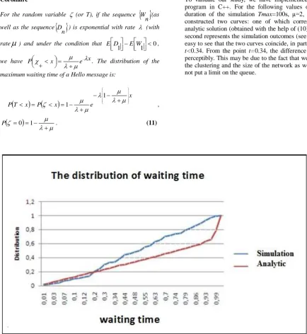
[image:4.595.54.489.78.551.2]

To validate our study, we have implemented a simulation program in C++. For the following values of parameters: duration of the simulation Tmax=100s, µ=2, λ=1, we have constructed two curves: one of which corresponds to the analytic solution (obtained with the help of (10)-(11)) and the second represents the simulation outcomes (see figure 1). It is easy to see that the two curves coincide, in particular for time t<0.34. From the point t=0.34, the difference appears more perceptibly. This may be due to the fact that we have omitted the clustering and the size of the network as well as we have not put a limit on the queue.

Fig 1: Comparison

4.

CONCLUDING REMARKS

Ad hoc networks, composed of wireless mobile nodes, can freely and dynamically self-organize and are without pre-existing infrastructure. In these communication systems, maintaining of the connectivity is a very big problem for which Hello messages are a solution.

In this work, we modeled the arrival of the Hello messages at a node as a random walk. By using the approach developed by Borovkov (1978), we obtained the exact expression of the waiting time distribution of a Hello message before its treatment by the reception node. With the help of this result, it is possible to calculate the TTL (Time To Live) of a message and the interval Hello (two essential parameters in the routing protocols).

5.

REFERENCES

[1] Basagni S., Conti M., Giordano S., and Stojmenovi I. 2004. ’Mobile Ad Hoc Networking’.IEEE Press John Wiley.

[2] Moy J. 1994 ’OSPF - Open Shortest Path First’. RFC 1583.

[3] Chakers I. D. and Beding-Royer E. M. 2002. ’The utility of hello messages for determining link connectivity’. Proceeding the 5th International Symposium on Wireless Personal Multimedia. Vol (2). 504-508.

IEEE International Symposium on Modeling, Analysis, and Simulation of Computer and Telecommunication Systems (MASCOTS 07). 9-14.

[5] Al Hanbali A., Ibrahim M., Simon V., Varga E., and Carreras I. 2008. ’A Survey of Message Diffusion Protocols in Mobile Ad hoc Networks’. Proceding of the 3rd International Conference on Performance Evaluation Methodologies and Tools.

[6] Groenevelt R., Nain P. and Koole G. 2005. ’The message delay in Ad hoc networks’. Performance Evaluation Journal. Vol(62). N°1-4. 210-228.

[7] Al Hanbali A. and Nain P. and Altman E. 2008. ’Performance of ad hoc networks with two-hop relay routing and limited packet lifetime (extented version)’. Performance Evaluation Journal. Vol(65). 463-483. [8] Diaz J., Petit J., and Serna M. 1998. ’Random geometric

problems on [0, 1]2’, Randomization and Approximation Techniques in Computer Science, vol. 1518 of Lecture Notes in Computer Science. 294–306. Springer-Verlag Berlin.

[9] Nemeth G. and Vattay G. 2002. ’Giant clusters in random ad hoc networks’. condmat/0211325.

[10]Newman M. E. J., Strogatz S. H., andWatts D. J. 2001. ’Random graphs with arbitrary degree distributions and their applications’. cond-mat/0007235.

[11]Gomez C. and Cuevas A. and Paradells J. 200). ’AHR: a two-state adaptive mechanism for link connectivity maintenance in AODV’. Proceeding of the 2nd international workshop on multi-hop mobile Ad Hoc networks: from theory to reality. 98-100.

[12]Giruka V. and Singhal M. 2005 Hello protocols for ad hoc networks : Overhead and accuracy trade-offs. Proceeding of the Sixth IEEE International Symposium on a World of Wireless Mobile and Multimedia Networks (WoWMoM’05). Vol (1). 354-361.