The Performance and Robustness of Interest Rate Rules in Models of the Euro Area

(1)

The Performance and Robustness of

Interest-Rate Rules in Models of the

Euro Area

Adalid, Ramon and Coenen, Gunter and McAdam, Peter

and Siviero, Stefano

10 February 2005

(2)

Interest-Rate Rules in Models of the Euro

Area

∗

Ram´on Adalid, G¨unter Coenen, Peter McAdam

European Central Bank

Stefano Siviero

Banca d’Italia

In this paper, we examine the performance and robust-ness of optimized interest-rate rules in four models of the euro area that diﬀer considerably in terms of size, degree of aggre-gation, relevance of forward-looking behavioral elements, and adherence to microfoundations. Our ﬁndings are broadly con-sistent with results documented for models of the U.S. econ-omy: backward-looking models require relatively more aggres-sive policies with, at most, moderate inertia; rules that are optimized for such models tend to perform reasonably well in forward-looking models, while the reverse is not necessarily true; and, hence, the operating characteristics of robust rules (i.e., rules that perform satisfactorily in all models) are heavily weighted towards those required by backward-looking models. JEL Codes: E31, E52, E58, E61

∗_{The paper summarizes the results of a project aimed at evaluating the}

performance of monetary policy rules in a number of small- to medium-scale models developed by Eurosystem staﬀ that have been regularly used for

pol-icy analysis. Helpful comments by Keith K¨uster, Sergio Nicoletti Altimari,

Athanasios Orphanides, Glenn Rudebusch, Frank Smets, Volker Wieland, John Williams, Raf Wouters; by participants at the ECB conference on “Monetary Policy and Imperfect Knowledge”; and by an anonymous referee are greatly appreciated. The opinions expressed are those of the authors and do not nec-essarily reﬂect views of the European Central Bank or the Banca d’Italia. Any remaining errors are the sole responsibility of the authors. Correspon-dence: Coenen: Directorate General Research, European Central Bank, e-mail: [email protected], homepage: www.guentercoenen.com; Adalid: Directorate General Research, European Central Bank, e-mail: ramon.adalid [email protected]; McAdam: Directorate General Research, European Central Bank, e-mail: [email protected]; Siviero: Economic Research Department, Banca d’Italia, e-mail: [email protected].

(3)

The design of robust monetary policy rules has attracted con-siderable interest in recent macroeconomic research. This interest largely reﬂects the increased awareness on the part of policymakers and academics alike that, when evaluating the possible consequences of alternative monetary policies, the existing uncertainties about the structure of the economy need to be given due account. As a re-sult, a large body of research has been oriented toward identifying the characteristics of monetary policy rules that perform “reason-ably well” across a range of potentially nonnested and competing

macroeconomic models.1 _{While this line of research has primarily}

focused on models of the U.S. economy, no systematic study has yet

been conducted for the euro area.2

In an attempt to fill this gap, we concentrate on the euro area and examine the performance and robustness of monetary policy rules us-ing a rather diverse set of macroeconomic models of the euro area economy. Such an examination seems particularly relevant as the single monetary policy of the European Central Bank (ECB) has to focus on the euro area as a whole, being a new and still relatively unexplored economic entity, and with models of the euro area having been developed only very recently. Specifically, our analysis relies on four models of the euro area economy that have been built by staff of the Eurosystem in recent years. These models differ considerably in terms of size, degree of aggregation, relevance of forward-looking behavioral elements, and adherence to microfoundations. They thus

cover a wide range of features that are a priori considered to be of

high relevance in the context of evaluating the robustness of

mone-tary policy rules.3 One of our main goals is to ascertain which of the

various features with respect to which these models diﬀer are of im-portance when designing rules suitable for model-based evaluations of monetary policy, and which features are, by contrast, arguably less important.

1

For an early claim in this respect see McCallum (1988).

2

Earlier studies of the performance of interest-rate rules across alternative models of the U.S. economy are provided in Bryant, Hooper, and Mann (1993) and Taylor (1999). More recent studies have been undertaken by Levin, Wieland,

and Williams (2003) and Levin and Williams (2003). The study of Cˆot´e et al.

(2002) focuses on models of the Canadian economy.

3

(4)

In terms of methodology, our analysis builds on recent work by Levin, Wieland, and Williams (1999, 2003) and Levin and Williams

(2003).4 _{This methodology involves implementing simple reaction}

functions describing the response of the short-term nominal interest rate to inflation and the output gap, either observed or forecast, and then optimizing over the respective response coefficients. The performance of these optimized interest-rate rules is then evaluated across alternative, potentially competing models with regard to their ability to stabilize inflation and output around their targets, while avoiding undue fluctuations in the nominal interest rate itself.

Of course, variables other than inflation and the output gap may enter the interest-rate rule, such as the exchange rate or monetary and financial-market indicators. However, the literature tends to sug-gest that including information variables of this kind in the policy rule yields relatively modest gains in model-based evaluations be-cause they are typically highly correlated with the interest rate itself or closely related with the measures of inflation and the output gap entering the rule (although this result may not hold in sufficiently complex models). Furthermore, simple rules with a feedback to a small set of variables are arguably more robust to model misspecifi-cation and uncertainty than rules based on a larger set of variables, which might overfit specific model characteristics.

From an institutional viewpoint, the advantage of simple interest-rate rules is clearly their transparency and, thus, the ease with which they may be communicated to and monitored by the outside world. While it is unlikely that monetary policymakers will follow their lit-eral execution, such rules may nonetheless be a useful benchmark for assessing the actual conduct of monetary policy. Likewise, from an empirical point of view, simple interest-rate rules seem to match the data well for the United States as well as a number of European countries (see Clarida, Gal´ı, and Gertler 1998). More recently, evi-dence for the euro area as a whole has been provided by Gerdesmeier and Roﬃa (2004).

4

(5)

The ﬁndings of our analysis are broadly consistent with the re-sults documented for models of the U.S. economy: backward-looking models require relatively more aggressive policies with, at most, mod-erate inertia; rules that are optimized for such models tend to per-form reasonably well in forward-looking models, while the reverse is not necessarily true; and, hence, the operating characteristics of robust rules (i.e., rules that perform satisfactorily in all models) are heavily weighted toward those required by backward-looking mod-els. In the course of collecting these results, we highlight a number of model features (notably, the degree of forward-lookingness) that play a crucial role in shaping the operating characteristics of opti-mized interest-rate rules. This in turn suggests that future empirical research that aims at casting additional light on these features may enhance the reliability and usefulness of interest-rate rules for model-based evaluations of monetary policy.

The remainder of this paper is organized as follows. Section 1 outlines the set of euro area models used in our analysis and illus-trates the implied differences in inflation and output-gap dynamics in response to a monetary policy shock. Section 2 briefly describes the methodology used for evaluating the performance of interest-rate rules and provides a set of optimized benchmark rules for each of the euro area models under examination. Section 3 evaluates the robust-ness of these benchmark rules when there is uncertainty about the true structure of the euro area economy, as represented by the coex-istence of possibly competing models, while section 4 identifies the operating characteristics of rules that attain satisfactory outcomes across the set of models used. Section 5 reports additional sensitivity analysis, and section 6 concludes.

1. The Models of the Euro Area

(6)

while forward-looking elements abound in the other two. All models are consistent with basic economic principles; however, there is only one in our set of models that is strictly based on the assumption of optimizing agents. Hence, the models under examination cover a fairly broad range of diﬀerent modeling strategies.

In the remainder of this section, we briefly present the four mod-els of the euro area and illustrate the implied differences in inflation and output-gap dynamics in response to a monetary policy shock.

1.1 An Outline of the Euro Area Models

1.1.1 The Coenen-Wieland Model

The Coenen-Wieland (CW) model (see Coenen and Wieland 2000) is a small-scale model of aggregate supply and aggregate demand that is designed to capture the broad characteristics of inﬂation and output dynamics in the euro area. Since its development, the model has been mainly used as a laboratory for evaluating the performance of alternative monetary policy strategies.

The supply side of the model incorporates price and wage stagger-ing, with wage setters negotiating long-term nominal wage contracts with reference to past contracts that are still in effect and future con-tracts that will be negotiated over the life of the current contract. If wage setters expect the output gap to be positive, they adjust the current contract wages upward, and vice versa. Consequently, inflation depends on its own leads and lags, excess-demand condi-tions, and transitory contract wage shocks—the latter representing “cost-push” shocks. There are two versions of the supply side that feature distinct types of staggered wage contracts: the nominal wage contracting specification due to Taylor (1980) and the relative real

wage contracting speciﬁcation by Fuhrer and Moore (1995).5 _The

two specifications differ with respect to the degree of inflation per-sistence that they induce, with Fuhrer-Moore-type contracts giving

5

(7)

more weight to past inﬂation developments. In this paper, the version

with Taylor-type contracts is used.6

A simple aggregate demand relationship relates the output gap (measured as the deviation of actual output from a smooth trend) to several lags of itself, the ex-ante long-term real interest rate, and a transitory demand shock. The long-term real rate is determined jointly by a term-structure relationship and the Fisher equation. The short-term nominal interest rate is the instrument of monetary pol-icy, and changes in the latter aﬀect aggregate demand through the impact on the ex-ante long-term real interest rate.

1.1.2 The Smets-Wouters Model

The Smets-Wouters (SW) model (see Smets and Wouters 2003) is an extended version of the standard New Keynesian dynamic stochastic general equilibrium (DSGE) model with sticky prices and wages. The model is estimated by Bayesian techniques using seven euro area macroeconomic time series: real gross domestic product (GDP), consumption, investment, employment, real wages, inﬂation, and the nominal short-term interest rate.

The model features three types of economic agents: households, firms, and the monetary policy authority. Households maximize a utility function with two arguments (goods and leisure) over an infi-nite life horizon. Consumption appears in the utility function relative to a time-varying external habit-formation variable. Labor is differ-entiated over households, so that there is some monopoly power over wages, which results in an explicit wage equation and allows for the

introduction of sticky nominal wages `a la Calvo (1983). Households

also rent capital services to ﬁrms and decide how much capital to ac-cumulate given certain capital adjustment costs. As the rental price of capital goes up, the capital stock can be used more intensively ac-cording to some cost schedule. Firms produce diﬀerentiated goods,

decide on labor and capital inputs, and set prices, again `a la Calvo

(1983). The Calvo model in both wage and price setting is augmented

6

(8)

by the assumption that those prices and wages that cannot be freely set are partially indexed to past inflation. Prices are therefore set as a function of current and expected real marginal cost, but are also influenced by past inflation. Real marginal cost depends on wages and the rental rate of capital. The short-term nominal interest rate

is the instrument of monetary policy.7

The stochastic behavior of the model is driven by ten exoge-nous shocks: five shocks arising from technology and preferences, three cost-push shocks, and two monetary policy shocks. The first set of shocks is assumed to follow first-order autoregressive processes, whereas the second set is assumed to follow serially uncorrelated pro-cesses. Consistent with the DSGE setup, potential output is defined as the level of output that would prevail under flexible prices and wages in the absence of cost-push shocks.

1.1.3 The Area-Wide Model

The Area-Wide Model (AWM; see Fagan, Henry, and Mestre 2001) is a medium-size structural macroeconomic model that treats the euro

area as a single economy.8 It has a long-run neoclassical equilibrium

with a vertical Phillips curve, but with some short-run frictions in price and wage setting and factor demands. Consequently, activity is demand-determined in the short run but supply-determined in the long run. In the latter, employment converges to a level consis-tent with the exogenously given level of equilibrium unemployment, and factor demands are consistent with the solution of the firms’ profit-maximization problem. Stock-flow adjustments are accounted for by, for example, the inclusion of a wealth term in consumption. At present, the treatment of expectations in the model is quite limited. With the exception of the exchange rate (determined by uncovered interest parity) and the long-term nominal interest rate (modeled by a term-structure relationship), the model embodies backward-looking expectations.

7

Extending the study of Coenen (2003), Angeloni, Coenen, and Smets (2003) utilize the SW model to analyze the design of monetary policy when the monetary policymaker is uncertain about the degree of nominal as well as real persistence. The results of this analysis conﬁrm the conclusions of the earlier study.

8

For an examination of optimal monetary policy in the context of the AWM

(9)

As to the mechanisms through which monetary policy affects the economy, aggregate demand in the AWM is presently influenced only by short-term real interest rates. Long-term nominal rates determine the government’s debt service but do not explicitly enter investment decisions. The expectations channel in principle allows monetary pol-icy to influence inflation via wage- and price-setting behavior. In ad-dition to these influences, further effects enter through the exchange rate. Apart from an indirect effect of exchange rates on domestic de-mand, there is also a direct exchange-rate effect on consumer price inflation through the price for imported goods. The output gap is defined as the ratio of actual output to potential output, which is based on an aggregate Cobb-Douglas production function with con-stant returns to scale and Hicks-neutral technical progress. For this, trend total factor productivity has been estimated within-sample by applying the Hodrick-Prescott filter to the Solow residual derived from the production function.

1.1.4 A Disaggregate Model of the Euro Area

(10)

the area-wide short-term nominal interest rate is the instrument of monetary policy.

As the model allows for simultaneous cross-country linkages, it was estimated with the three-stage least-squares (3SLS) method us-ing data on inflation, output, and nominal interest rates. Not all cross-country terms are significant in all equations. This results in a clear causal pattern, with the German economy affecting the other two comparatively more, and with the Italian economy be-ing essentially recursive. Furthermore, the estimation results indi-cate that there exists a significant degree of heterogeneity among

the three economies included in the model.9 Accordingly, the

re-sults in Angelini et al. (2002) suggest that monetary policy eﬀective-ness may be considerably enhanced if country-speciﬁc information is used.

1.2 Differences in Monetary Policy Transmission

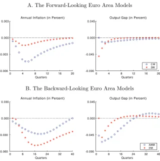
Figure 1 provides a comparison of the effects of an unexpected one-quarter tightening of monetary policy by 100 basis points in the four different models of the euro area, with the monetary policymaker following the interest-rate rule proposed by Taylor (1993) thereafter. Panel A of the figure depicts the dynamic responses of annual infla-tion and the output gap for the largely forward-looking models (CW and SW), while panel B shows the responses for the predominantly backward-looking models (AWM and DM).

Qualitatively, the tightening of policy has the same consequences in the four models. As the short-term nominal interest rate rises un-expectedly, demand falls short of potential and inflation falls below the monetary policymaker’s target, with the dynamic adjustment being drawn out lastingly. Quantitatively, however, the responses ex-hibit some noticeable differences. Most importantly, the disinflation effect is considerably larger and more persistent in the backward-looking models with the timing of the peak effect on inflation notice-ably delayed relative to that on the output gap. By contrast, in the

9

(11)

[image:11.612.128.448.175.497.2]

Figure 1. Responses to an Interest-Rate Shock (100 Basis Points) under Taylor’s Rule

A. The Forward-Looking Euro Area Models

0 4 8 12 16 20 -0.006

-0.003 0.000 0.003

Annual Infl ation (in Percent)

Quarters

0 4 8 12 16 20 -0.090

-0.045 0.000 0.045

Output Gap (in Percent)

Quarters

CW SW

B. The Backward-Looking Euro Area Models

0 8 16 24 32 40 -0.060

-0.030 0.000 0.030

Annual Infl ation (in Percent)

Quarters

0 8 16 24 32 40 -0.090

-0.045 0.000 0.045

Output Gap (in Percent)

Quarters

AWM DM

forward-looking models, the timing of the peak effect on inflation is much closer to that on the output gap, with the reversion to base of both inflation and the output gap being more rapid and smoother. Differences in the responses of the output gap, notably in the initial periods, largely reflect differences in the employed output-gap con-cepts. Overall, this suggests that the degree of forward-lookingness is of utmost relevance for explaining the differences in inflation and output-gap dynamics across models.

(12)

a given interest-rate rule may perform quite diﬀerently in terms of inﬂation and output-gap stabilization, depending on the characteris-tics of the particular euro area model used. Hence, it is evident why monetary policymakers should be concerned about the design of the interest-rate rule to be used in model-based analyses.

2. Evaluating the Performance of Interest-Rate Rules

We now proceed to describe the methodology that we will use to evaluate the stabilization performance of alternative monetary poli-cies across our set of models of the euro area economy. Our starting point is an evaluation of simple interest-rate rules that respond to outcomes or forecasts of annual inﬂation and the output gap and al-low for inertia due to dependence on the lagged short-term nominal interest rate.

2.1 The Methodology

Following the approach in Levin, Wieland, and Williams (2003), we consider a three-parameter family of simple interest-rate rules,

it=ρ it−₁+ (1−ρ) (r∗+ Et[ ˜πt+θ] ) +αEt[ ˜πt+θ−π∗] +βEt[yt+κ],

whereitdenotes the short-term nominal interest rate,r∗ is the

equi-librium real interest rate, ˜πt=pt−pt−₄ is the annual inﬂation rate,

π∗

denotes the monetary policymaker’s inﬂation target, andytis the

output gap.10 Under rational expectations, the operator Et[·]

in-dicates the model-consistent forecast of a particular variable, using

information available in period t.11 The integer parameters θ and

κ denote the length of the forecast horizons for inﬂation and the

output gap, respectively. This speciﬁcation accommodates

forecast-based rules (with forecast horizonsθ, κ >0) as well as outcome-based

10

Even in the case where the multicountry model DM is used, both inﬂation and the output gap are to be interpreted as area-wide variables, reﬂecting the assumption that the policymaker is concerned with area-wide developments.

11

(13)

rules (θ=κ= 0) and simpliﬁes to the one proposed by Taylor (1993)

ifθ=κ= 0,ρ= 0 and α=β = 0.5.12

For ﬁxed inﬂation and output-gap forecast horizons θandκ, the

above family of interest-rate rules is deﬁned by the response

coef-ﬁcients ρ, α, and β. The coeﬃcients α and β represent the

policy-maker’s short-term reaction to inﬂation in deviation from target and

the output gap, respectively, while ρ determines the inertia of the

interest-rate response, commonly interpreted as the desired degree of policy “smoothing.” The latter plays an important role for model-based evaluations of interest-rate rules. In particular, the degree to which the optimal policy in any given model embodies smoothing tends to depend largely on the expectation formation mechanism embedded in that model. Typically, if expectations are backward

looking, values ofρ at or above unity can perform poorly since they

may engender undampened oscillations in the model economy due to instrument instability (see, e.g., Rudebusch and Svensson 1999 and Batini and Nelson 2001). By contrast, models with largely forward-looking expectations, notably small optimizing New Keynesian mod-els, tend to favor a comparatively high degree of smoothing because the inertial adjustment of the short-term interest rate enables the policymaker to steer expectations and thereby to stabilize the econ-omy more eﬀectively.

In our evaluation of the stabilization performance of variants of the above family of interest-rate rules, we assume that the mone-tary policymaker has a standard loss function equal to the weighted sum of the unconditional variances of inﬂation, the output gap, and changes in the short-term nominal interest rate,

L= Var[πt] +λVar[yt] +µVar[ ∆it].

Here, inﬂation is measured by the annualized one-quarter inﬂation

rate,πt= 4 (pt−pt−₁). The weightλ≥0 refers to the policymaker’s

preference for reducing output variability relative to inﬂation

vari-ability, and the weight µ ≥ 0 on the variability of changes in the

12

In the special case withρ = 1, the rule represents a ﬁrst-diﬀerence rule, a

class of rules that Levin, Wieland, and Williams (2003) advocate as being robust when examining the performance of simple interest-rate rules across a set of dis-tinct models of the U.S. economy—none of them, however, being fully backward-looking. Orphanides and Williams (2002) emphasize that ﬁrst-diﬀerence rules are

(14)

short-term nominal interest rate, ∆it = it−it−1, reﬂects a desire

to avoid undue ﬂuctuations in the nominal interest rate itself.13

Es-tablishing this loss function is consistent with the assumption that the policymaker aims at stabilizing inﬂation around the inﬂation

tar-getπ∗

and actual output around potential, with the concern regard-ing excessive interest-rate variability typically justiﬁed by ﬁnancial

stability considerations.14

For ﬁxed inﬂation and output-gap forecast horizons θandκ, the

three-parameter family of interest-rate rules deﬁned above is

opti-mized by minimizing the policymaker’s loss functionLwith respect

to the coeﬃcients ρ, α, and β. In this context, we repeatedly need

to compute the unconditional variances of the models’ endogenous variables for a given interest-rate rule. In preparation for these com-putations, we ﬁrst identify the series of historical shocks that would be consistent with the alternative models under rational expecta-tions. Based on the covariance matrix of the historical shocks, it is then possible to calculate the unconditional covariance matrix of the endogenous variables for any given interest-rate rule by applying standard methods to the reduced-form solution of the model

includ-ing that rule.15

In the subsequent analysis, we will consider four alternative values for the relative weight on output-gap variability, namely

λ = 0,1/3,1, and 3. Regarding the weight on the variability of

interest-rate changes, we will concentrate the analysis on a ﬁxed

value of µ = 0.10. We shall brieﬂy discuss additional results for a

lower weight of µ = 0.01 in the sensitivity analysis in section 5.

There, we will also report on results for interest-rate rules that only

13

For an explicit derivation of the policymaker’s loss functionLfrom quadratic

intertemporal preferences, the reader is referred to Rudebusch and Svensson

(1999). In Svensson’s terminology, the case ofλ=µ= 0 corresponds to “strict”

inflation targeting, while “flexible” inflation targeting is characterized byλ, µ >0

(see Svensson 1999).

14

It is recognized that it would be beneﬁcial to use a welfare criterion de-rived as an approximation of the representative agent’s utility function (see, e.g., Rotemberg and Woodford 1997). The weights in this approximate welfare crite-rion would be functions of the parameters of the structural model itself. However, to the extent that the models used in this paper, with the exception of the SW model, are lacking microfoundations, a well-deﬁned welfare criterion does not exist.

15

(15)

allow for a response to lagged inﬂation and the lagged output gap;

that is, with θ=κ=−1. Such rules have been proposed as a proxy

for actual policymaking in “real time” (see McCallum 1988).

2.2 The Performance of Optimized Benchmark Rules

As benchmarks for evaluating the performance of simple interest-rate rules across our set of models, we focus on two types of rules:

outcome-based rules with θ =κ = 0, and forecast-based rules that

relate the interest rate to the one-year-ahead forecast of inﬂation and

the contemporaneous output gap withθ= 4 and κ= 0.

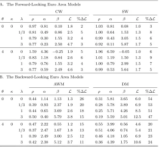
Table 1 reports the optimized response coeﬃcients of the two types of rules for the four diﬀerent models of the euro area economy

and for alternative values of the preference parameter λ, together

with an indication of their stabilization performance. The latter is measured by the value of the policymaker’s loss function yielded

under the rule optimized for a particular modelL and alternatively,

in relative terms, as the percentage-point diﬀerence of the loss under the optimized rule from the loss under the fully optimal policy for

that model, %∆L.16 Panel A in table 1 indicates the results for the

largely forward-looking models (CW and SW), while panel B shows the results for the predominantly backward-looking models (AWM and DM).

We start with the results for the forward-looking models in panel A and observe that, regardless of the policymaker’s prefer-ence for output stabilization, the optimized rules are characterized by a substantial degree of interest-rate smoothing, as captured by the

high coeﬃcient on the lagged interest rate,ρ. Interestingly, with a low

weight on output stabilization and, in particular, with the inﬂation forecast horizon extending one year into the future, the magnitude

of ρ tends to exceed unity, notably for the SW model. This feature

is commonly referred to as “super-inertia” in the interest rate. Not surprisingly, as the weight on output stabilization increases, the

co-efficient on the output gap,β, rises while the coefficient on inflation,

16

For the CW and SW models, as well as the AWM, the fully optimal policy cor-responds to the optimal policy under commitment. See Finan and Tetlow (1999) for details on computing the optimal policy under commitment for large rational expectations models using AIM. Details regarding the unconditional variability of the individual target variables underlying the calculation of the loss function,

(16)

[image:16.612.127.451.171.469.2]

Table 1. The Stabilization Performance of Optimized Interest-Rate Rules

CW SW

θ κ λ ρ α β L _%∆L ρ α β L _%∆L

0 0 0 0.97 0.81 0.10 1.8 2 1.03 0.81 0.08 1.0 3 1/3 0.81 0.49 0.86 2.5 5 1.00 0.64 1.53 1.3 8 1 0.79 0.30 1.55 3.2 4 0.99 0.43 3.05 1.5 6 3 0.77 0.23 2.50 4.7 3 0.92 0.11 5.87 1.7 5

4 0 0 1.59 4.36 −0.25 1.9 5 1.96 6.59 −0.05 1.0 6 1/3 0.83 1.18 0.84 2.6 6 1.01 1.19 1.50 1.3 9 1 0.79 0.76 1.55 3.2 4 1.00 0.79 2.99 1.5 7 3 0.77 0.59 2.49 4.6 3 0.99 0.53 5.64 1.7 5

AWM DM

θ κ λ ρ α β L %∆L ρ α β L %∆L

0 0 0 0.44 1.14 1.13 1.3 26 0.31 5.81 3.65 6.0 54 1/3 0.39 0.93 2.37 1.9 20 0.28 5.78 3.89 6.9 53 1 0.44 0.65 3.69 2.6 18 0.25 5.71 4.26 8.5 51 3 0.50 0.40 5.79 3.8 15 0.19 5.59 5.01 12.5 47

4 0 0 0.47 2.22 0.55 1.2 15 0.55 3.99 0.56 4.6 20 1/3 0.37 2.47 1.67 1.8 13 0.51 4.06 0.74 5.4 21 1 0.39 2.49 3.00 2.5 12 0.46 4.18 1.05 6.9 23 3 0.42 2.38 5.12 3.7 11 0.36 4.39 1.75 10.6 24

Note: For each choice of the inﬂation and output-gap forecast horizons (θ and

κ), for each preference parameter (λ) and for each model, this table indicates

the optimized interest-rate response coeﬃcients (ρ,α, and β), the value of the

policymaker’s loss function (L), and the percentage-point diﬀerence of the latter

from the loss under the fully optimal policy (%∆L).

α, falls. As regards the stabilization performance of the optimized

(17)

simple optimized interest-rate rule rather than the fully optimal policy. The value of the policymaker’s loss function never rises by more than 9 percentage points. We also observe that there is no dis-cernible stabilization gain from following forecast-based as opposed to outcome-based rules.

Turning to the backward-looking models in panel B, a number of diﬀerences are noteworthy. First, the optimized interest-rate rules

embody only a mild degree of smoothing, with ρ varying between

0.4 and 0.5 for the AWM and between 0.2 and 0.6 for the DM. This discrepancy largely reﬂects the fact that expectations, notably those determining long-term interest rates, do not play a dominant role in either model. Thus, there is no scope for increasing the eﬀectiveness of monetary policy by an inertial adjustment of the short-term rate.

Second, the optimized response coeﬃcients α and β are typically

quite a bit larger than for the forward-looking models, in particular for the DM. This mirrors the fact that, in backward-looking models, inflation and the output gap are much harder to stabilize and, as a result, the policymaker has to respond more aggressively to any signs of rising inflation and cumulating output gaps. Third, when compared with the outcomes under the fully optimal policies, the stabilization performance of simple interest-rate rules deteriorates quite substantially, albeit less strongly for the AWM. In the extreme case when the policymaker does not attach any weight to output stabilization, the loss under the optimized outcome-based rule ex-ceeds the loss associated with the fully optimal policy by more than 50 percentage points for the DM, while the loss differs by about 25

percentage points for the AWM.17 In the case of the AWM, the

rel-atively poor performance of simple optimized rules is likely due to the model’s fairly high degree of structural detail and its rather com-plex dynamics (see Finan and Tetlow [1999] for a similar observation

based on the Federal Reserve Board’s FRB/US model).18 _Similarly,

17

Evidently, while the values of the loss function obtained for the AWM are comparable with those yielded in the forward-looking models, the losses for the DM are quite a bit larger.

18

(18)

the DM departs from the rest of the models to the extent that it is the only model in which the three largest euro area economies are modeled separately. Fourth, contrary to the results for the forward-looking models, there are substantial gains in performance from using forecast-based rather than outcome-based rules, with the maximum gain equal to 11 percentage points for the AWM and 34 percentage

points for the DM (in the case of λ = 0). We attribute these

im-provements in performance to the information-encompassing nature of forecast-based rules, with the inﬂation forecast incorporating in-formation about incipient risks to future inﬂation arising from a pos-sibly larger set of underlying determinants (see Batini and Haldane 1999) and the transmission lag of monetary policy (see Batini and Nelson 2001).

3. Evaluating the Robustness of Interest-Rate Rules

In the previous section, we implicitly assumed that the policymaker knows the “true” model of the euro area economy when optimizing variants of the three-parameter family of interest-rate rules for any given model. While the optimized rules typically succeeded in sta-bilizing inﬂation and output satisfactorily for that given model, we now proceed to analyze to what extent the optimized rules are robust to model uncertainty, in the sense of also performing reasonably well across the other, possibly competing models of the euro area.

3.1 The Performance of Optimized Rules Across Models

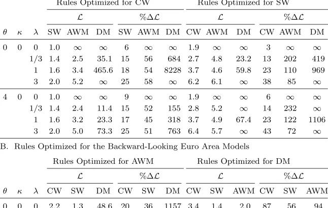
Table 2 summarizes our ﬁndings regarding the stabilization per-formance of the optimized benchmark rules documented in table 1 above across our set of models. Here, performance is measured

by the value of the policymaker’s loss function, L, and by the

percentage-point diﬀerence of the latter from the loss under the

fully optimal policy, %∆L, when the rule optimized for any

partic-ular model m is evaluated in the possibly competing model n=m.

Panel A in table 2 reports the ﬁndings for the rules optimized for

(19)

[image:19.612.126.449.195.400.2]

Table 2. The Robustness of Optimized Interest-Rate Rules in Models of the Euro Area

A. Rules Optimized for the Forward-Looking Euro Area Models

Rules Optimized for CW Rules Optimized for SW

L _%∆L L _%∆L

θ κ λ SW AWM DM SW AWM DM CW AWM DM CW AWM DM

0 0 0 1.0 ∞ ∞ 6 ∞ ∞ 1.9 ∞ ∞ 3 ∞ ∞

1/3 1.4 2.5 35.1 15 56 684 2.7 4.8 23.2 13 202 419 1 1.6 3.4 465.6 18 54 8228 3.7 4.6 59.8 23 110 969

3 2.0 5.2 ∞ ₂₅ ₅₈ ∞ _6.2 _6.1 ∞ ₃₈ ₈₅ ∞

4 0 0 1.0 ∞ ∞ 9 ∞ ∞ 1.9 ∞ ∞ 6 ∞ ∞

1/3 1.4 2.4 11.4 15 52 155 2.8 5.2 ∞ 14 232 ∞

1 1.6 3.2 23.3 17 45 318 3.7 4.9 67.4 23 122 1106 3 2.0 5.0 73.3 25 51 763 6.4 5.7 ∞ 43 72 ∞

B. Rules Optimized for the Backward-Looking Euro Area Models

Rules Optimized for AWM Rules Optimized for DM

L _%∆L L _%∆L

θ κ λ CW SW DM CW SW DM CW SW AWM CW SW AWM

0 0 0 2.2 1.3 48.6 20 36 1157 3.4 1.4 2.0 87 56 94 1/3 2.7 1.5 222.2 11 24 4859 3.8 1.7 2.3 58 39 43 1 3.5 1.7 ∞ ₁₄ ₂₃ ∞ _4.7 _2.2 _2.7 ₅₃ ₅₅ ₂₄

3 ME 2.0 ∞ _ME ₂₃ ∞ _6.8 _3.2 _3.9 ₅₂ ₉₇ ₁₇

4 0 0 2.3 1.3 11.8 25 40 205 2.5 1.3 1.3 40 37 27 1/3 2.7 1.6 15.2 13 30 238 2.8 1.7 2.1 16 35 30 1 3.4 1.8 20.2 13 31 261 3.7 2.3 3.1 20 64 41 3 5.2 2.1 34.3 16 31 303 5.8 3.6 5.2 29 120 56

κ), for each preference parameter (λ) and for each model, this table indicates the

value of the policymaker’s loss function (L) and the percentage-point diﬀerence

of the latter from the loss under the fully optimal policy (%∆L), when the rule

optimized for modelmis evaluated in modeln=m. The notation “ME” indicates

that the implemented rule yields multiple equilibria; the notation “∞” indicates

that the implemented rule results in instability.

the forward-looking models, while panel B documents those for the backward-looking ones.

(20)

and vice versa. For example, with θ = κ = 0 and λ = 1/3, imple-menting the CW-based rule in the SW model leads to an increase in the loss function of about 15 percentage points, relative to the loss associated with the fully optimal policy for the SW model. When compared to the performance of the interest-rate rule optimized for the SW model itself (see table 1), the loss increases by about 7 per-centage points. Similarly, when implementing the SW-based rule in the CW model, the increase in the loss function amounts to 13 and 8 percentage points, depending on the benchmark for comparison. By contrast, when evaluating the CW- and SW-based rules in the backward-looking models, the performance of monetary policy tends to deteriorate quite substantially. For the AWM, the loss increases by about 50 percentage points relative to the fully optimal policy when CW-based rules are implemented and by more than 100 percentage points on average for SW-based rules. The deterioration is found to be particularly dramatic if the policymaker puts zero weight on out-put stabilization since the CW- and SW-based rules do not succeed in stabilizing the AWM any longer. Finally, when evaluated in the DM, the performance of CW- and SW-based rules is even worse, generating even higher increases in relative losses and resulting in instability more often.

Turning to the rules optimized for the backward-looking models in panel B, we observe that the AWM-based rules typically result in reasonable stabilization outcomes when evaluated in the CW or

the SW model. The exception is the outcome-based rule for λ= 3,

which yields multiple equilibria when implemented in the CW model. By contrast, the AWM-based rules do not perform satisfactorily in the DM and may occasionally even generate instability. Finally, the DM-based rules result in a substantial deterioration in the perfor-mance of monetary policy when evaluated in any of the three other models, although the deterioration exceeds 100 percentage points only in exceptional cases. Interestingly, for forecast-based rules, the deterioration is found to be somewhat more benign.

Based on these results, we conclude that simple interest-rate rules that are designed for the predominantly backward-looking euro area models tend to perform reasonably well in the largely

forward-looking models, while the reverse is not necessarily true.19 The

19

(21)

fault-tolerance analysis undertaken in the next section will cast some further light on the reasons underlying these ﬁndings.

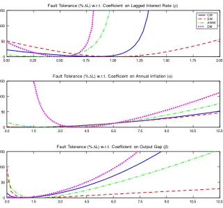
3.2 A Fault-Tolerance Analysis of Optimized Rules

Fault-tolerance analysis of optimized interest-rate rules, as proposed by Levin and Williams (2003), is deemed to provide useful insights into the reasons that underlie our earlier ﬁndings. Fault-tolerance analysis is a concept borrowed from engineering and involves, in the present context, appraising the increase in the loss function that re-sults when a single parameter of an optimized interest-rate rule is varied, holding the other parameters constant at their optimized

val-ues. A highly fault tolerant model is one for which the parameters

of the rule may vary over a relatively broad range of values without resulting in a large deterioration of its performance. By contrast, an intolerant model would be a model whose performance deterio-rates dramatically as soon as one deviates even modestly from some optimized parameter value (i.e., the loss function exhibits strong curvature with respect to suboptimal variations in some parameter). Clearly, if one is dealing with a set of relatively tolerant models, there is a fair chance to ﬁnd a robust policy rule. If all models are intolerant, then a robust rule may not exist.

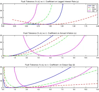
Figure 2 depicts the fault tolerances of our four models for the

case θ = κ = 0 and λ = 1/3 (i.e., for the outcome-based rules

obtained with a moderate weight on output stabilization).20 Each

curve shows the percentage-point change in the policymaker’s loss function under the optimized rule as a single parameter is varied, with its minimum of zero attained at the optimized value itself. As can be seen in the ﬁgure, while any single parameter may be varied over a relatively broad range of values without deteriorating dra-matically the performance of the individual model concerned, there

are no obvious overlapping regions of high mutual fault tolerance

for all four models under examination and for all three policy-rule parameters at the same time.

other predominantly backward-looking model), suggesting that the choice of the degree of aggregation is also a relevant factor in shaping the results.

20

For other values of the preference parameterλ,the results are qualitatively

(22)

[image:22.612.128.448.176.471.2]

Figure 2. Fault-Tolerance Analysis of Outcome-Based Interest-Rate Rules

0.00 0.25 0.50 0.75 1.00 1.25 1.50 1.75 2.00 0

50 100 150

Fault Tolerance (%∆L) w.r.t. on Lagged Interest Rate (ρ)

CW SW AWM DM

0.0 1.5 3.0 4.5 6.0 7.5 9.0 10.5 12.0 0

50 100 150

Fault Tolerance (%∆L) w.r.t. Coefficient Coefficient

on Annual Inf lation (α)

0.0 1.5 3.0 4.5 6.0 7.5 9.0 10.5 12.0 0

50 100 150

Fault Tolerance (%∆L) w.r.t. Coefficient on Output Gap (β)

Note: Forλ= 1/3 and for each model, the ﬁgure indicates the percentage-point

change in the policymaker’s loss function (%∆L) under the optimized

outcome-based interest-rate rule (θ = κ = 0) as a single parameter (ρ, α, or β) of the

optimized rule is varied, holding the other two parameters ﬁxed at their respective optimized values.

Regarding the fault tolerances with respect to the smoothing

coeﬃcient ρ (displayed in the upper panel of the ﬁgure), the two

forward-looking models perform best when ρ is close to unity, while

the performance for both the AWM and DM deteriorates quite markedly in this region, eventually resulting in instrument instability

for the DM. In contrast, the AWM prefers aρcoeﬃcient of somewhat

(23)

of ρ in this region, however, tend to yield indeterminate equilibria for the forward-looking models, notably for the CW model. With

respect to the response coeﬃcient α (depicted in the middle panel),

the forward-looking models and the AWM seem mutually tolerant to

variations in α in the region of close to 0 to 2.5. The DM, however,

behaves very diﬀerently in its optimal prescription forα, demanding

a signiﬁcantly higher value of about 6, but with the curvature of the loss function in that region being modest. By contrast, as shown in the lower panel, a comfortable region of relatively high mutual tolerance seems to exist with respect to variations in the response

coeﬃcient β in the range of 2 to 4. While the DM favors a strong

response to the output gap in the range of 2 to 7.5, the three other models perform satisfactorily as a group for coeﬃcients in the range of 0.5 to 4, with the CW model constraining the upper bound of this range.

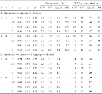
Interestingly, as shown in ﬁgure 3, the four models exhibit consid-erably larger regions of mutual fault tolerance when the policymaker

follows a forecast-based rule with θ = 4 and κ = 0. In this case,

variations in ρ in the range of 0.4 to 0.7 result in a reasonable

per-formance of all four models. Similarly, there are regions of mutual

tolerance with respect to variations in α and β, the regions being

centered at 3.5 and 1, respectively.

4. Designing Robust Interest-Rate Rules

The fault-tolerance analysis in the previous section has provided an indication under which circumstances a robust interest-rate rule might exist for our set of euro area models. However, to the extent that fault-tolerance analysis rests on suboptimal variations in a sin-gle policy-rule parameter, holding ﬁxed the other parameters at their optimized values, we ﬁnally proceed to use a more formal approach that allows taking into account the interaction among all policy-rule parameters to identify the operating characteristics of interest-rate rules that are likely to yield satisfactory outcomes across our models.

(24)

[image:24.612.128.449.173.472.2]

Figure 3. Fault-Tolerance Analysis of Forecast-Based Interest-Rate Rules

0.00 0.25 0.50 0.75 1.00 1.25 1.50 1.75 2.00 0

50 100 150

Fault Tolerance (%∆L) w.r.t. Coefficient on Lagged Interest Rate (ρ)

CW SW AWM DM

0.0 1.5 3.0 4.5 6.0 7.5 9.0 10.5 12.0 0

50 100 150

Fault Tolerance (%∆L) w.r.t. Coefficient on Annual Inf lation (α)

0.0 1.5 3.0 4.5 6.0 7.5 9.0 10.5 12.0 0

50 100 150

Fault Tolerance (%∆L) w.r.t. Coefficient on Output Gap (β)

Note: Forλ= 1/3 and for each model, the ﬁgure indicates the percentage-point

change in the policymaker’s loss function (%∆L) under the optimized

forecast-based interest-rate rule (θ= 4,κ= 0) as a single parameter (ρ,α, orβ) of the

optimized rule is varied, holding the other two parameters ﬁxed at their respective optimized values.

minimizing a weighted average of the loss functions associated with the individual models,

¯

L=

m∈M

ωmLm,

where ωm denotes the weight attached to any given model m ∈

M ⊆ {CW,SW, AWM,DM} with ωm > 0 and ωm = 1. For

(25)

[image:25.612.125.450.172.472.2]

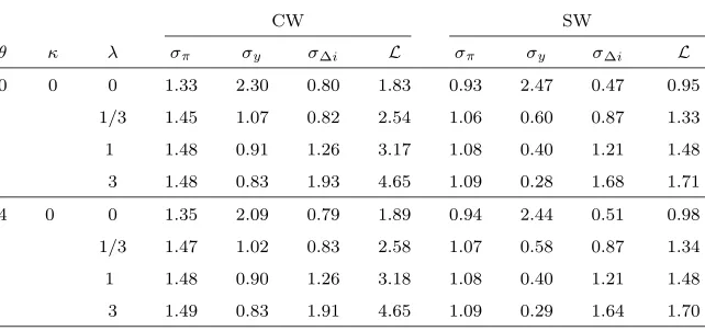
Table 3. The Stabilization Performance of Bayesian Robust Interest-Rate Rules

L_m _{generated in} _%∆L_m _{generated in}

θ κ λ ρ α β CW SW AWM DM CW SW AWM DM A. Optimization Across All Models

0 0 0 0.54 3.38 2.28 2.6 1.3 1.6 6.4 46 38 58 64

1/3 0.58 3.22 2.71 3.1 1.5 2.3 7.2 28 22 46 60

1 0.58 3.21 3.33 3.9 1.8 3.2 8.8 28 30 45 58

3 0.54 3.33 4.48 5.8 2.4 4.8 13.2 29 50 47 56

4 0 0 0.60 3.28 0.49 2.3 1.2 1.3 4.7 26 33 25 22

1/3 0.62 3.27 1.16 2.7 1.5 2.0 5.7 11 22 25 28

1 0.60 3.46 1.90 3.4 1.8 2.7 7.5 10 29 25 34

3 0.54 3.76 3.16 5.0 2.3 4.1 12.1 11 42 24 43

B. Optimization Across All Aggregate Models

0 0 0 0.71 0.76 0.55 2.1 1.1 1.4 14 24 33

1/3 0.63 0.64 1.72 2.6 1.4 2.0 8 17 24

1 0.64 0.42 2.78 3.3 1.6 2.7 8 17 22

3 0.64 0.37 4.37 5.0 1.9 4.0 10 18 20

4 0 0 0.72 1.26 0.39 2.2 1.2 1.2 20 29 20

1/3 0.64 1.40 1.46 2.6 1.5 1.9 8 19 17

1 0.62 1.38 2.56 3.3 1.7 2.6 8 19 17

3 0.62 1.42 4.17 4.9 2.0 3.8 9 20 16

κ) and for each preference parameter (λ), this table indicates the jointly

opti-mized interest-rate response coeﬃcients (ρ, α, and β), the contribution of the

individual modelmto the policymaker’s loss function (Lm), and the

percentage-point diﬀerence of this contribution from the loss under the fully optimal policy

(%∆Lm).

loss function when the policymaker has uniform prior beliefs as to

which model in M is a plausible representation of the euro area

economy.

(26)

performance of these rules yielded in the individual models. Here, performance is measured as the contributions of the individual

mod-els to the value of the policymaker’s overall loss function,Lm, and as

the percentage-point diﬀerence of these contributions from the losses

under the fully optimal policies, %∆Lm.

Starting with the outcome-based rules with θ= κ = 0, it turns

out that the jointly optimized (that is,Bayesian robust) policies are

heavily weighted toward those demanded by the DM, with the op-timized interest-rate response coefficients close to those implied by the DM alone (see table 1). Specifically, the Bayesian robust poli-cies prescribe a degree of interest-rate smoothing in the range of 0.5 to 0.6, while the responses to inflation and the output gap are rather aggressive. The response to inflation is relatively stable at around 3, while the response to the output gap varies quite a bit, namely in the range of 2 to 4, depending on the weight given to output stabilization. In light of the fault-tolerance analysis reported above, this outcome is not really surprising, since, in the absence of regions of high mutual tolerance with respect to some parame-ter, the least tolerant model is supposed to be most influential in shaping the operating characteristics of the robust policy with

re-spect to that parameter.21 Nevertheless, the robust policies perform

reasonably well in all four models, notably if a sensible weight is given to output-gap stabilization, as can be seen when comparing the outcomes under the robust policies with the performance mea-sures reported in table 1. In fact, the increase in the reported losses never exceeds 50 percentage points, even if the sole policy objective

is to stabilize inﬂation (i.e., for λ = 0), with the deterioration in

performance obviously smallest for the DM due to its inﬂuential role in shaping the operating characteristics of the robust policies. This ﬁnding is broadly consistent with the results documented in Levin and Williams (2003) for a set of models of the U.S. economy includ-ing the backward-lookinclud-ing model of Rudebusch and Svensson (1999). Also in this study, the contours of the robust policies are found to be

21

(27)

heavily weighted towards those demanded by the backward-looking model.

Turning to the forecast-based rules with θ = 4 and κ = 0, the

performance of Bayesian robust policies is found to be even more satisfactory across models. Yet again, this ﬁnding is not surprising in light of the fault-tolerance analysis above indicating the existence of regions of relatively high mutual tolerance for all three parameters. However, the optimized parameters of the robust rules appear to be largely inﬂuenced by the DM again.

To the extent that the robust policies for the full set of mod-els are heavily weighted toward the policies demanded by the DM, panel B of table 3 also reports results obtained when optimizing across all aggregate models, but excluding the DM. In this case, the robust policies are characterized by a uniformly higher degree of interest-rate smoothing (in a range of 0.6 to 0.7) and, overall, by less aggressive responses to inﬂation and the output gap. As expected, the performance of the robust policies designed for the two forward-looking models (CW and SW) and the AWM alone ap-pears more favorable across these models when compared to the performance under the robust rules designed for the full set of models.

5. Sensitivity Analysis

Now we brieﬂy summarize some additional sensitivity analysis re-garding the results presented above. First, we consider the

impli-cations of changing the weight µ on the variability of interest-rate

changes in the policymaker’s loss function. For the preceding

anal-ysis we have chosen a weight of µ = 0.1, which has been widely

employed in policy evaluation exercises like ours. As shown in

ta-ble B-1 in the appendix, with a weight of µ= 0.01 on interest-rate

(28)

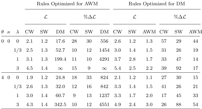
despite these changes in the operating characteristics of the opti-mized rules, we observe—by comparing the relative performance measures reported in table B-2 with those in table 2—that the ro-bustness properties of the optimized rules are broadly unaﬀected if

the weight on interest-rate variability is lowered toµ= 0.01. Finally,

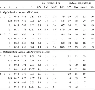
as documented in table B-3, jointly optimized interest-rate rules are yet again found to be weighted toward the DM, but with the rela-tively favorable performance of robust forecast-based rules being less clear-cut.

Regarding the sensitivity of our results with respect to using a

real-time information set with θ = κ = −1, table C-1 shows that

the performance of real-time-based rules tends to deteriorate rela-tive to that of outcome-based rules. For the more backward-looking models, this deterioration is rather pronounced (up to 69 and 34 percentage points for the AWM and the DM, respectively, depend-ing on the weight given to output stabilization). Similarly, as shown in table C-2, the robustness of real-time-based rules tends to be in-ferior to that of outcome-based ones, resulting in a somewhat larger deterioration of performance across models. Finally, as indicated in table C-3, the performance of robust real-time-based rules is slightly inferior across models as well.

6. Conclusions

(29)

those required by the backward-looking models. Nevertheless, the Bayesian robust policies identified in such a way perform reasonably well in all four models, notably if a sensible weight is given to out-put stabilization. Especially, we find that a forecast-based rule that relates the short-term interest rate to the one-year-ahead forecast of inflation and the contemporaneous output gap and (importantly) that allows for only a moderate degree of inertia, attains reasonable outcomes.

While other model features such as variable and country cover-age and adherence to microfoundations are apparently of relevance as well, the nature of the expectation formation mechanism embed-ded in the various models seems to be of key importance for ex-plaining our results. This in turn suggests that future research that aims at casting light on the empirical relevance of forward-looking behavioral elements in macroeconomic models may enhance the re-liability and usefulness of interest-rate rules for model-based evalu-ations of monetary policy. Of course, in the case that a policy rule prescribed to set the interest rate in response to forecasts of fu-ture inﬂation, we assumed in our analysis that these forecasts hap-pened to be consistent with the structure of the particular model in which the performance of the forecast-based rule was evaluated. Sim-ilarly, the measure of the output gap used when evaluating the rule was consistent with the output-gap concept employed in that par-ticular model. To the extent that the monetary policymaker faces uncertainty regarding the reliability of the inﬂation forecast itself or the correct measurement of the output gap, these additional sources of uncertainty may heighten the risks associated with

re-lying too heavily on a rule optimized for any particular model.22

Extensions of our study along these directions are left for future research.

22

(30)

[image:30.612.127.448.223.374.2]

Appendix

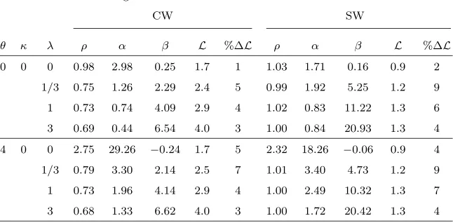
Table A. Detailed Results for the Optimized Interest-Rate Rules

CW SW

θ κ λ σπ σy σ∆i L σπ σy σ∆i L

0 0 0 1.33 2.30 0.80 1.83 0.93 2.47 0.47 0.95

1/3 1.45 1.07 0.82 2.54 1.06 0.60 0.87 1.33

1 1.48 0.91 1.26 3.17 1.08 0.40 1.21 1.48

3 1.48 0.83 1.93 4.65 1.09 0.28 1.68 1.71

4 0 0 1.35 2.09 0.79 1.89 0.94 2.44 0.51 0.98

1/3 1.47 1.02 0.83 2.58 1.07 0.58 0.87 1.34

1 1.48 0.90 1.26 3.18 1.08 0.40 1.21 1.48

3 1.49 0.83 1.91 4.65 1.09 0.29 1.64 1.70

AWM DM

θ κ λ σπ σy σ∆i L σπ σy σ∆i L

0 0 0 1.09 1.57 1.04 1.30 2.15 1.68 3.69 5.97

1/3 1.07 1.17 1.74 1.90 2.17 1.60 3.62 6.86

1 1.07 0.91 2.50 2.59 2.22 1.50 3.59 8.45

3 1.07 0.69 3.52 3.79 2.36 1.36 3.68 12.48

4 0 0 1.04 1.59 1.01 1.19 1.89 1.58 3.29 4.64

1/3 1.02 1.16 1.69 1.78 1.90 1.51 3.24 5.44

1 1.03 0.90 2.43 2.46 1.95 1.43 3.23 6.87

3 1.04 0.69 3.42 3.65 2.07 1.31 3.34 10.56

Note: For each choice of the inﬂation and output-gap forecast horizons (θandκ),

for each preference parameter (λ), and for each model, this table indicates the

unconditional standard deviations of the target variables (σπ,σy, andσ∆i) and

(31)

[image:31.612.126.449.203.362.2]

Table B-1. The Stabilization Performance of Optimized Interest-Rate Rules Generated with a Lower Weight of

µ= 0.01 on Interest-Rate Variability

CW SW

θ κ λ ρ α β L %∆L ρ α β L %∆L

0 0 0 0.98 2.98 0.25 1.7 1 1.03 1.71 0.16 0.9 2

1/3 0.75 1.26 2.29 2.4 5 0.99 1.92 5.25 1.2 9

1 0.73 0.74 4.09 2.9 4 1.02 0.83 11.22 1.3 6

3 0.69 0.44 6.54 4.0 3 1.00 0.84 20.93 1.3 4

4 0 0 2.75 29.26 −0.24 1.7 5 2.32 18.26 −0.06 0.9 4

1/3 0.79 3.30 2.14 2.5 7 1.01 3.40 4.73 1.2 9

1 0.73 1.96 4.14 2.9 4 1.00 2.49 10.32 1.3 7

3 0.68 1.33 6.62 4.0 3 1.00 1.72 20.42 1.3 4

AWM DM

θ κ λ ρ α β L _%∆L ρ α β L _%∆L

0 0 0 0.17 3.05 3.00 1.1 24 0.11 13.83 8.33 3.8 41

1/3 0.42 2.03 6.57 1.4 12 0.02 13.24 9.11 4.8 42

1 0.51 1.37 9.71 1.6 9 0.00 11.88 9.65 6.4 42

3 0.55 0.84 14.55 2.0 6 0.00 9.94 10.22 10.4 41

4 0 0 0.23 6.76 1.16 1.0 11 0.39 10.58 1.53 2.9 9

1/3 0.30 5.57 4.69 1.3 5 0.27 10.43 2.30 3.8 12

1 0.37 4.53 8.08 1.6 4 0.15 10.28 3.33 5.2 16

3 0.44 3.53 13.10 2.0 4 0.00 9.83 5.12 8.8 19

κ), for each preference parameter (λ), and for each model, this table indicates

the optimized interest-rate response coeﬃcients (ρ, α, andβ), the value of the

(32)

[image:32.612.124.452.403.580.2]

Table B-2. The Robustness of Optimized Interest-Rate Rules Generated with a Lower Weight of µ= 0.01 on

Interest-Rate Variability

L %∆L L %∆L

θ κ λ SW AWM DM SW AWM DM CW AWM DM CW AWM DM

0 0 0 0.9 ∞ ∞ 3 ∞ ∞ 1.7 ∞ ∞ 4 ∞ ∞

1/3 1.3 1.7 17.6 12 36 420 2.6 1.7 ∞ 13 34 ∞

1 1.4 1.9 97.4 13 29 2046 3.6 1.9 ∞ 31 29 ∞

3 1.5 2.5 ∞ 17 30 ∞ 6.5 2.2 ∞ 67 16 ∞

4 0 0 0.9 ∞ ∞ ₄ ∞ ∞ _1.7 ∞ ∞ ₆ ∞ ∞

1/3 1.3 1.6 27.3 12 30 704 2.6 1.8 ∞ ₁₃ ₄₃ ∞

1 1.3 1.8 30.3 12 21 567 3.5 1.8 ∞ ₂₅ ₂₃ ∞

3 1.5 2.4 90.2 16 23 1125 6.3 2.3 ∞ ₆₃ ₁₈ ∞

L %∆L L %∆L

θ κ λ CW SW DM CW SW DM CW SW AWM CW SW AWM

0 0 0 2.1 1.2 17.6 28 30 556 2.6 1.2 1.3 57 29 44

1/3 2.5 1.3 52.7 10 12 1454 3.0 1.4 1.5 31 26 19

1 3.1 1.3 199.4 11 10 4291 3.7 2.8 1.7 33 47 14

3 4.5 1.4 ∞ 15 9 ∞ 5.4 2.5 2.2 39 92 17

4 0 0 1.9 1.2 24.8 18 33 824 2.1 1.2 1.1 27 30 15

1/3 2.6 1.3 32.0 12 16 842 3.3 1.4 1.5 41 26 21

1 3.0 1.4 60.7 9 13 1237 3.3 1.7 2.0 17 45 33

3 4.3 1.4 342.5 10 12 4551 4.9 2.4 3.0 26 88 54

Note: For each choice of the inﬂation and output-gap forecast horizons (θandκ),

for each preference parameter (λ), and for each model, this table indicates the

value of the policymaker’s loss function (L) and the percentage-point diﬀerence

of the latter from the loss under the fully optimal policy (%∆L), when the rule

optimized for modelmis evaluated in modeln=m. The notation “∞” indicates

(33)

[image:33.612.127.449.190.496.2]

Table B-3. The Stabilization Performance of Bayesian Robust Interest-Rate Rules Generated with a Lower

Weight of µ= 0.01 on Interest-Rate Variability

L_mgenerated in %∆L_m generated in

θ κ λ ρ α β CW SW AWM DM CW SW AWM DM

A. Optimization Across All Models

0 0 0 0.42 8.54 5.81 2.3 1.1 1.2 3.9 39 25 32 46

1/3 0.39 7.86 6.69 2.7 1.3 1.6 5.0 17 18 27 47

1 0.33 7.63 8.02 3.3 1.6 2.0 6.7 20 31 36 49

3 0.21 7.54 10.31 4.9 2.0 2.9 11.0 26 60 53 49

4 0 0 0.47 8.62 1.19 2.2 1.2 1.1 3.9 33 28 14 45

1/3 0.45 8.14 3.17 2.5 1.3 1.4 4.7 10 17 13 38

1 0.38 8.31 4.93 3.0 1.5 1.7 6.2 10 23 16 37

3 0.26 8.56 7.56 4.3 1.8 2.3 10.3 12 39 22 39

0 0 0 0.56 2.73 1.53 2.0 1.1 1.2 21 21 32

1/3 0.59 1.74 4.78 2.5 1.2 1.4 7 11 14

1 0.63 1.04 7.03 3.0 1.3 1.7 6 10 12

3 0.61 0.65 10.37 4.1 1.4 2.1 6 11 10

4 0 0 0.64 4.78 0.81 2.1 1.1 1.1 29 25 16

1/3 0.57 3.77 4.07 2.5 1.3 1.3 8 13 7

1 0.59 3.09 6.63 3.0 1.3 1.6 6 11 7

3 0.58 2.66 10.17 4.1 1.4 2.1 6 12 7

κ) and for each preference parameter (λ), this table indicates the jointly

(34)

Table C-1. The Stabilization Performance of Optimized Interest-Rate Rules Based on a Real-Time Information

Set with θ=κ=−1

CW SW

λ ρ α β L _%∆L ρ α β L _%∆L

0 0.95 0.79 0.11 1.8 2 1.02 0.79 0.08 1.0 3

1/3 0.76 0.48 0.91 2.6 6 0.98 0.56 1.38 1.4 11

1 0.74 0.29 1.58 3.2 5 0.96 0.35 2.62 1.6 12

3 0.72 0.28 2.43 4.8 6 0.98 0.00 3.44 1.9 20

AWM DM

λ ρ α β L %∆L ρ α β L %∆L

0 0.42 0.99 1.11 1.4 34 0.17 6.07 4.26 7.3 88

1/3 0.27 0.82 2.16 2.2 40 0.13 6.06 4.46 8.3 85

1 0.26 0.54 3.19 3.4 55 0.07 6.02 4.77 10.1 81

3 0.25 0.34 4.60 6.1 84 0.00 5.79 5.30 14.8 74

Note: For each preference parameter (λ) and for each model, this table indicates

the optimized interest-rate response coeﬃcients (ρ, α, andβ), the value of the

(35)

Table C-2. The Robustness of Optimized Interest-Rate Rules Based on a Real-Time Information Set with

θ=κ=−1

L %∆L %L %∆L

λ SW AWM DM SW AWM DM CW AWM DM CW AWM DM

0 1.0 ∞ ∞ 6 ∞ ∞ 1.9 ∞ ∞ 4 ∞ ∞

1/3 1.4 2.8 66.7 18 80 1388 2.8 13.7 68.0 14 766 1417

1 1.7 4.5 ∞ 24 103 ∞ 3.8 21.4 ∞ 23 872 ∞

3 2.2 8.5 ∞ 38 157 ∞ ME ∞ ∞ ME ∞ ∞

L %∆L L %∆L

λ CW SW DM CW SW DM CW SW AWM CW SW AWM

0 2.2 1.3 94.5 20 36 2345 3.5 1.6 2.5 93 71 140

1/3 2.7 1.6 ∞ ₁₁ ₂₉ ∞ _3.9 _1.9 _3.2 ₆₁ ₅₀ ₁₀₆

1 ME 1.9 ∞ _ME ₃₈ ∞ _4.8 _2.3 _4.6 ₅₉ ₆₇ ₁₁₀

3 ME 2.6 ∞ _ME ₅₈ ∞ _7.1 _3.5 _8.0 ₅₇ ₁₁₅ ₁₄₃

Note: For each preference parameter (λ) and for each model, this table indicates

the value of the policymaker’s loss function (L) and the percentage-point

diﬀer-ence of the latter from the loss under the fully optimal policy (%∆L), when the

rule optimized for modelm is evaluated in modeln =m. The notation “ME”

indicates that the implemented rule yields multiple equilibria; the notation “∞”

(36)

[image:36.612.125.450.178.373.2]

Table C-3. The Stabilization Performance of Bayesian Robust Interest-Rate Rules Based on a Real-Time

Information Set with θ=κ=−1

L_m generated in %∆L_m generated in

λ ρ α β CW SW AWM DM CW SW AWM DM A. Optimization Across All Models

0 0.41 3.62 2.52 2.7 1.3 1.9 7.8 48 44 81 103

1/3 0.41 3.57 2.88 3.2 1.6 2.8 8.7 31 30 80 95

1 0.39 3.62 3.46 4.1 2.0 4.3 10.6 33 44 95 89

3 0.32 3.75 4.54 6.2 2.9 7.4 15.5 37 76 125 82

0 0.65 0.78 0.61 2.1 1.2 1.4 14 26 40

1/3 0.51 0.64 1.70 2.6 1.5 2.3 8 22 44

1 0.47 0.57 2.68 3.3 1.8 3.5 9 29 60

3 0.41 0.59 4.10 5.1 2.4 6.2 13 45 88

Note: For each preference parameter (λ), this table indicates the jointly

(%∆Lm).

References

Anderson, Gary S., and George R. Moore. 1985. “A Linear Algebraic

Procedure for Solving Linear Perfect Foresight Models.”

Eco-nomics Letters 17:247–52.

Angelini, Paolo, Paolo Del Giovane, Stefano Siviero, and Daniele Terlizzese. 2002. “Monetary Policy Rules for the Euro Area: What Role for National Information?” Temi di Discussione No. 457, Banca d’Italia (December).

Angeloni, Ignazio, G¨unter Coenen, and Frank Smets. 2003.

“Persis-tence, the Transmission Mechanism and Robust Monetary

Pol-icy.” Scottish Journal of Political Economy 50:527–49.

Batini, Nicoletta, and Andrew Haldane. 1999. “Forward-Looking

Rules for Monetary Policy.” In Monetary Policy Rules, ed. John

(37)

Batini, Nicoletta, and Edward Nelson. 2001. “Optimal Horizons for

Inﬂation Targeting.”Journal of Economic Dynamics and Control

25:891–910.

Blanchard, Olivier J., and Charles Kahn. 1980. “The Solution of

Linear Diﬀerence Models Under Rational Expectations.”

Econo-metrica 48:1305–11.

Bryant, Ralph C., Peter Hooper, and Catherine L. Mann, eds. 1993. Evaluating Policy Regimes: New Research in Empirical

Macroe-conomics. Washington, DC: Brookings Institution.

Calvo, Guillermo A. 1983. “Staggered Prices in a Utility-Maximizing

Framework.” Journal of Monetary Economics 12:383–98.

Chari, V. V., Patrick J. Kehoe, and Ellen R. McGrattan. 2000. “Sticky Price Models of the Business Cycle: Can the

Con-tract Multiplier Solve the Persistence Problem?” Econometrica

68:1151–80.

Clarida, Richard, Jordi Gal´ı, and Mark Gertler. 1998. “Monetary

Policy Rules in Practice: Some International Evidence.”

Euro-pean Economic Review 42:1033–67.

Coenen, G¨unter. 2003. “Inﬂation Persistence and Robust Monetary

Policy Design.” ECB Working Paper No. 290, European Central Bank (November).

Coenen, G¨unter, and Volker Wieland. 2000. “A Small Estimated

Euro Area Model with Rational Expectations and Nominal Rigidities.” ECB Working Paper No. 30, European Central Bank

(September), forthcoming in European Economic Review.

Cˆot´e, Denise, John Kuszczak, Jean-Paul Lam, Ying Liu, and Pierre St-Amant. 2002. “The Performance and Robustness of Simple Monetary Policy Rules in Models of the Canadian Economy.” Technical Report 92, Bank of Canada.

Dieppe, Alistair, Keith K¨uster, and Peter McAdam. 2004. “Optimal

Monetary Policy Rules for the Euro Area: An Analysis Using the Area Wide Model.” ECB Working Paper No. 360, European

Central Bank (May), forthcoming inJournal of Common Market

Studies.

Fagan, Gabriel, Jerome Henry, and Ricardo Mestre. 2001. “An Area-Wide Model (AWM) for the Euro Area.” ECB Working Paper

No. 42, European Central Bank (January), forthcoming in

Eco-nomic Modelling.

(38)

Two Examples.” Finance and Economics Discussion Series, 99-51, Board of Governors of the Federal Reserve System (October). Fuhrer, Jeﬀrey C., and George R. Moore. 1995. “Inﬂation

Persis-tence.” Quarterly Journal of Economics 110:127–60.

Gerdesmeier, Dieter, and Barbara Roﬃa. 2004. “Empirical Estimates

of Reaction Functions for the Euro Area.” Swiss Journal of

Eco-nomics and Statistics 140:37–66.

Giannoni, Marc P. 2002. “Does Model Uncertainty Justify Caution?

Robust Monetary Policy in a Forward-Looking Model.”

Macro-economic Dynamics 6:111–44.

Giannoni, Marc P., and Michael Woodford. 2002. “Optimal Inter-est Rates: I. General Theory.” NBER Working Paper No. 9419 (December).

Hansen, Lars P., and Thomas J. Sargent. 2002. “Robust Control and Model Uncertainty in Macroeconomics.” Unpublished Book Manuscript, University of Chicago and Hoover Institution. King, Robert, and Alexander Wolman. 1999. “What Should the

Monetary Authority Do When Prices Are Sticky?” In Monetary

Policy Rules, ed. John B. Taylor. Chicago: NBER and University

of Chicago Press.

Levin, Andrew T., Volker Wieland, and John C. Williams. 1999. “Robustness of Simple Policy Rules under Model Uncertainty.”

In Monetary Policy Rules, ed. John B. Taylor, 263–99. Chicago:

NBER and University of Chicago Press.

Levin, Andrew T., Volker Wieland, and John C. Williams. 2003. “The Performance of Forecast-Based Monetary Policy Rules

un-der Model Uncertainty.” American Economic Review 93:622–45.

Levin, Andrew T., and John C. Williams. 2003. “Robust Monetary

Policy with Competing Reference Models.”Journal of Monetary

Economics 50:945–75.

McCallum, Bennett T. 1988. “Robustness Properties of a Rule for

Monetary Policy.”Carnegie Rochester Conference Series on

Pub-lic PoPub-licy 29:173–204.

Monteforte, Libero, and Stefano Siviero. 2002. “The Economic Con-sequences of Euro-Area Modeling Shortcuts.” Temi di Discus-sione No. 458, Banca d’Italia (December).

Onatski, Alexei, and James H. Stock. 2002. “Robust Monetary Policy under Model Uncertainty in a Small Model of the U.S. Economy.”