General Integral Control Design via Singular Perturbation Technique

(1)

http://dx.doi.org/10.4236/ijmnta.2014.34019

General Integral Control Design via Singular

Perturbation Technique

Baishun Liu, Xiangqian Luo, Jianhui Li

Academy of Naval Submarine, Qingdao, China

Email: [email protected], [email protected], [email protected]

Received 10 August 2014; revised 8 September 2014; accepted 15 September 2014

This work is licensed under the Creative Commons Attribution International License (CC BY). http://creativecommons.org/licenses/by/4.0/

Abstract

This paper proposes a systematic method to design general integral control with the generic inte-grator and integral control action. No longer resorting to an ordinary control along with a known Lyapunov function, but synthesizing singular perturbation technique, mean value theorem, stabil-ity theorem of interval matrix and Lyapunov method, a universal theorem to ensure regionally as well as semi-globally asymptotic stability is established in terms of some bounded information. Its highlight point is that the error of integrator output can be used to stabilize the system, just like the system state, such that it does not need to take an extra and special effort to deal with the integral dynamic. Theoretical analysis and simulation results demonstrated that: general integral controller, which is tuned by this design method, has super strong robustness and can deal with nonlinearity and uncertainties of dynamics more forcefully.

Keywords

General Integral Control, Nonlinear Control, Robust Control, General Integrator, General Integral Action, Singular Perturbation Method, Output Regulation

1. Introduction

Integral control [1] plays an important role in practice because it ensures asymptotic tracking and disturbance rejection when exogenous signals are constants or planting parametric uncertainties appear. However, integral control design is not trivial matter because it depends on uncertain parameters and disturbances. Therefore, it is of important significance to develop the design method on the integral control.

(2)

sliding mode technique and feedback linearization technique were presented by [2]-[4], respectively. The main shortage of these design methods proposed by literature [2]-[4] is that they were all achieved by using a kind of particular integrator and linear integral action, which are a serious obstruction to design a high performance integral controller. In addition, general concave integral control [5], general convex integral control [6], con-structive general bounded integral control [7] and the generalization of the integrator and integral control action [8] were all developed by resorting to an ordinary control along with a known Lyapunov function. This results in that design methods presented by [5]-[8] are all suspended in midair. Thus, it is a very valuable and challenging problem to establish a solid foundation for designing general integral control with the generic integrator and integral control action.

Motivated by the cognition above, this paper proposes a systematic method to design general integral control with the generic integrator and integral control action. The main contributions are that: 1) By mean value theo-rem, the nonlinear actions in the subsystem and integral dynamics are all reformulated as the linear forms on the interval matrix such that stability theorem of interval matrix can be used to deal with them; 2) The error of inte-grator output can be used to stabilize the system, just like the system state, such that it does not need to take an extra and special effort to deal with the integral dynamic; 3) No longerresorting to an ordinary control along with a known Lyapunov function, but synthesizing singular perturbation technique, mean value theorem, stabil-ity theorem of interval matrix and Lyapunov method, a universal theorem to ensure regionally as well as semi- globally asymptotic stability is established in terms of some bounded information.Consequently, this universal theorem is not suspended in midair but is developed with a solid foundation. Moreover, simulation results showed that general integral controller, which is tuned by this design method, has superstrong robustness and can deal with nonlinearity and uncertainties of dynamics more forcefully.

Throughout this paper, we use the notation λ_m

( )

A and λ_M

( )

A to indicate the smallest and largest eigen-values, respectively, of a symmetric positive defined bounded matrix A x

( )

, for any x∈Rn. The norm of vector x is defined as x = x xT , and that of matrix A is defined as the corresponding induced norm A = λ_M

( )

A AT . For two n m× matrices A and B, A≥B denotes element-by-element inequality. A family of interval matrices is defined as,

( )

A A, A Rn m× :A A A

Λ =_ ∈ ≤ ≤ _

where A=   a_ij and A=   a_ij are fixed matrices. The family Λ is described geometrically as hyperrec-tangle in the space n m

R× of the coefficients a_ij. We say that a n n

R× family matrix Λ is Hurwitz stable if every A∈ Λ is Hurwitz stable.

The remainder of the paper is organized as follows: Section 2 describes the system under consideration, as-sumption and definition. Section 3 addresses the design method. Example and simulation are provided in Sec-tion 4. Conclusions are presented in SecSec-tion 5.

2. Problem Formulation

Consider the following controllable nonlinear system,

( )

(

)

(

)

,

, , , ,

x

z

x f x z

z f x z w g x z w u

=  

= +





 (1)

where n

x∈R and _z_∈_Rm_{are the states;} m

u∈R is the control input; l

w∈R is a vector of unknown constant parameters and disturbances. The partial derivative of function f_x on

( )

x z, is bounded in the control domain

n m

x z

D ×D ⊂R ×R , and fx

( )

0, 0 =0. The functions, fz and g are continuous in

(

x z w, ,

)

on the control do-

main n m l

x z w

D ×D ×D ⊂R ×R ×R . We want to design a control law, u such that x t

( )

→0 and z t

( )

→0 as t→ ∞.

Assumption 1: There is a unique pair

(

0, 0,u₀

)

that satisfies the equations,

(

)

(

)

0

(3)

Assumption 2: No loss of generality, suppose that the functions f_z

(

x z w, ,

)

and g x z w

(

, ,

)

satisfies the following inequalities,

(

, ,

)

(

0, 0,

)

z z

x z

z z f f

f x z w − f w ≤l x +l z (3)

(

, ,

)

0

g ≥g x z w ≥ >g (4)

(

, ,

)

(

0, 0,

)

gx gz

g x z w −g w ≤l x +l z (5)

for all x∈D_x, z∈D_z and w∈D_w. where

z

x f

l ,

z

z f

l , l_gx and l_gz are all positive constants.

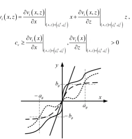
Definition 1: F a b c x_φ

(

_φ, _φ, _φ,

)

with a_φ >0, b_φ >0 and x∈Rn denotes the set of all continuously diffe-rential increasing functions [8],

( )

T

1 1 2 2 n n

x x x x

φ _{= }φ φ  φ _

such that

( )

0 0

φ = ,

( )

:

i xi bφ xi R xi aφ

φ ≥ ∀ ∈ >

( )

(

)

[image:3.595.125.466.393.695.2] [image:3.595.206.426.458.689.2]

d _i _i d _i 0 _i 1, 2, , c_φ ≥ φ x x > ∀ ∈x R i=  n . where  stands for the absolute value.

Figure 1 depicts the example curves of one component of the functions belonging to the function set F_φ. For instance, for all x∈R, the functions, ax

(

a>0

)

, tanh

( )

x , arcsinh

( )

x and so on, all belong to function set

F_φ.

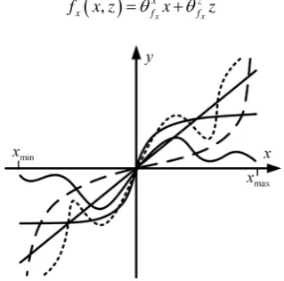
Definition 2: F c x zv

(

v, ,

)

with cv >0,

n x

x∈D ⊂R and m z

z∈D ⊂R denotes the set of all integrable functions [8],

( )

T

1 2

, , , n ,

v x z = _v x z v x z  v x z _

such that

( )

(

)

( )

(

)

, , , ,

, ,

,

x z x z

i i i i

i i

i

x z x z

v x z v x z

v x z x z

x ₌_{ς ς} z ₌_{ς ς}

∂ ∂

= +

∂ ∂ ,

( )

(

)

( )

(

)

, , , ,

, 0

x z x z

i i i i

i i

v

x z x z

v x v x

c

x ₌_{ς ς} z ₌_{ς ς}

∂ ∂

≥ >

∂ ∂

(4)

[image:4.595.233.393.534.692.2]

hold for all i=1, 2,,n, and

(

ς ς_ix, _iz

)

is a point on the line segment connecting

( )

x z, to the origin.

Figure 2 depicts the example curves of one component of the functions belonging to the function set F_v. For instance, for all x∈ −

(

1,1

)

, and z∈ −

(

1,1

)

, the functions, x+3z, tanh

( )

x +sinh

( )

z , sinh

(

x+2z

)

, and so on, all belong to the function set F_v.

3. Control Design

In general, integral controller comprises three components: the stabilizing controller, the integral control action and the integrator, and then the general integral controller can be given as,

( )

(

)

( ) ( )

1

,

x z

u K x K z K

v x z

σ

ε φ σ

σ β σ

−

 = − + +

 

=

 (6) where K_x, K_z and K_σ are the m × n, m × m and m × m gain matrices, respectively; σ_i =β σ_i

( ) ( )

_i v x z_i , ;

( )

0

i i

c_β ≥β σ >

(

i=1, 2,,m

)

;

ε

is a positive constant; the functions φ

( )

• and v

( )

• belong to the func-tion sets F_φ and F_v, respectively.

Thus, substituting (6) into (1), obtain the augmented system,

( )

(

)

(

)

(

( )

)

( ) ( )

,

, , , ,

, x

z x z

x f x z

z f x z w g x z w K x K z K

v x z

σ

ε ε φ σ

σ β σ = 

 ₌ ₋ ₊ ₊

 

= 

  

(7)

By Assumption 1 and choosing ε−1K_σ to be nonsingular and large enough, and then setting z=0 and 0

x= =z of the system (7), we obtain,

(

0, 0,

)

( )

0 z

(

0, 0,

)

g w Kσφ σ =εf w (8) Therefore, we ensure that there is a unique solution σ₀, and then

(

0, 0,σ₀

)

is a unique equilibrium point of the closed-loop system (7) in the domain of interest. At the equilibrium point, x= =z 0, irrespective of the value of w.

Now, by Mean Value Theorem for each component of the vector function f_x

( )

x z, , we have,

( )

(

)

( )

(

)

, , , ,

, ,

,

x z x z

i i i i

xi xi

xi

x z x z

f x z f x z

f x z x z

x ₌_{ς ς} z ₌_{ς ς}

∂ ∂

= +

∂ ∂

where i=1, 2,,n and

(

ς ς_ix, _iz

)

is a point on the line segment connecting

( )

x z, to the origin. For convenience, the function, f_x

( )

x z, can be written as a compact formulation, that is,

( )

,

x x

x z

x f f

f x z =θ x+θ z

(5)

where,

1 2 1 2

T T

,

x x x xn x x x xn

x x x x z z z z

f f f f f f f f

θ =_θ θ _ θ _ θ =_θ θ _ θ _ .

Thus, by the bound of partial derivative of function f_x on

( )

x z, , we can ensure that the matrices

x

x f

θ and

x

z f

θ belong to the families of interval matrices, respectively, that is,

, , ,

x x x x x x

x x x z z z

f f f f f f

θ ∈_θ θ _ θ ∈_θ θ _.

In the same way, we obtain,

( ) ( )

, ,

( ) ( )

0

(

0

)

x z

v v

v x z x z _ϕ

β σ =θ +θ φ σ −φ σ =θ σ σ−

Therefore, by c_β ≥β σ_i

( )

_i >0, and Definitions 1 and 2, we have, , , , , ,

x x x z z z

v v v v v v φ φ φ

θ ∈_θ θ _ θ ∈_θ θ _ θ _{∈ }θ θ _,

and then substituting them and (8) into (7), obtain,

(

) (

)

1

0 0 0 0 0

x x

x z

f f

x z z z z

x z

v v

x x z

z gK x gK z gK f f g g g f

x z

σ φ

θ θ

ε θ σ σ ε ε

σ θ θ

−  = +  _{= −} ₋ ₋ ₋ ₊ ₋ ₋ ₋   = +     (9) where

(

, ,

)

, 0

(

0, 0,

)

,

(

, ,

)

, and 0

(

0, 0,

)

z z z z

f = f x z w f = f w g=g x z w g =g w .

Now, defining η=

[

x σ−σ₀

]

T, y=z−h(η),

) ( )

(η =−K−1K x−K−1K_σθ_φσ−σ₀

h _z _x _z ,

and then the closed-loop system (9) can be rewritten as,

( )

(

)

d , d y A y y y y η

η η δ

εδ η τ

 = +

 

= Λ +   (10) where 1 1 1 1

x x x

x z z

f f z x f z

x z z

v v z x v z

K K K K

A

K K K K

σ φ

θ θ θ θ

− − − −  − −  =   − −     ,

( )

0

0 0 x z f z v y y η θ δ θ  _{  } =           , z gK

Λ = − , τ =t ε, and

(

) (

)

1

( )

0 0 0 0

,

y y fz fz g g g fz h

δ η ₌ ₋ ₋ ₋ − ₋  η _.

In the absence of δ_η

( )

y and δ η_y

(

,y

)

, the asymptotic stability of the closed-loop system (10) can be achieved by designing the interval matrices A and Λ are all Hurwitz stable [9]. Thus, by linear system theory, two quadratic Lyapunov functions,

( )

T

A

V_η η =η Pη (11)

( )

T

y

(6)

can be obtained, respectively. Where P_A and PΛ are the solutions of Lyapunov equations P AA +A PT A = −I

and _P T_P _I

ΛΛ + Λ Λ = − , respectively. It is obvious that PA and PΛ are all interval matrices, that is, ,

A A A

P ∈ P P _ and P_Λ∈ P P_Λ, _Λ_.

Based on the Lyapunov Functions (11) and (12), a composite Lyapunov function candidate [10] for the closed-loop system (10) can be written as,

(

,

) (

1

) ( )

_y

( )

0 1

V η y = −d V_η η +dV y < <d (13) Obviously, Lyapunov function candidate (13) is positive define. Therefore, our task is to show that its time derivative along the trajectories of the closed-loop system (10) is negative define, which is given by,

(

) (

) ( )

( )

(

)

T

(

)

T

( ) (

) ( )

T T T

(

)

T

(

)

, 1

1 1 1 , , .

y

A A y y A

V y d V dV y

d d P y d y P dy y dy P y d y P y

η

η η

η η η δ δ η Λδ η δ η

= − +

= − − + − + − − + +

  

(14)

By definitions of h

( )

η and φ σ

( )

, we have,

( )

1 1

( )

z x z

h η = −K K x− −K K− _σφ σ

( )

φ σ

( )

φ σ

( ) ( ) ( )

v x z,

φ σ σ β σ

σ σ

∂ ∂

= =

∂ ∂

 _

and then substituting φ σ

( )

, x, and z= +y h

( )

η into h

( )

η , and using Assumptions 2, and Definitions 1 and 2, we have,

(

,

)

_y y_y

y y y

η

δ δ

δ η ≤γ η γ+ (15)

In addition, by ,

x x x

z z z

f f f

θ _{∈ }θ θ _, z z, z

v v v

θ _{∈ }θ θ _ and definition of δη

( )

y , obtain,

( )

y

y _η y

η δ

δ ≤γ (16)

where y η δ γ , y y δ

γ , and γ_δy_η are all positive constants. Substituting (15) and (16) into (14), obtain,

(

)

(

)

2

(

1

)

2

(

)

T

1 2

, 1 2 1

V η y ≤ − −d η −d ε− −γ y + −d β +dβ y η = −ξ ξQ (17)

where

( )

(

)

(

)

(

)

(

)

1 , 2 , T 1 2 1 1 2

, Max ,

2 , ,

1 1

. 1

A A A

y

A

P P P

y y P P P

y y

P P P

P y

d d d

Q

d d d

η

δ η η

η δ

δ

β γ

γ γ ξ η

β β

β β ε γ

Λ Λ Λ

  ∈  Λ   ∈  − = = = = = = _ _ − − −   =   − − −    

The right-hand side of the inequality (17) is a quadratic form, which is negative define when,

(

)

(

₁

)

(

)

2

1 2

1−d d ε− −γ > 1−d β +dβ (18) which is equivalent to,

(

)

(

)

(

)

2

1 2

1

1 1

d

d d

d d d d

ε ε

γ β β

− < =

(7)

By the dependence of ε_d on d, it is obvious that the maximum value of ε_d occurs at d∗ =β β β₁

(

₁+ ₂

)

[10] and is given by,

1 2

1 4 d

ε ε

γ β β

∗_< ₌

+ (20)

It follows that the origin of closed-loop system (10) is asymptotically stable for all ε ε< ∗. Consequently, by 0

η= and y=0, we have x=0, σ σ= ₀ and z=h

( )

η =0. This means that the closed-loop system (7) is asymptotically stable, too. This established the following Theorem.

Theorem 1: Under Assumptions 1 and 2, if there exist gain matrices K_x, K_z and Kσ such that the inter-val matrices A and Λ are all Hurwitz stable and the following inequality,

( )

(

)

(

0, 0,

)

m g Km σ aφ f w

λ φ >ε (21)

holds to ensure that there exist positive constants ε_d and ε∗,and then

(

0, 0,σ₀

)

is an exponentially stable equilibrium point of the closed-loop system (7) for all ε ε< ∗. Moreover, if all assumptions hold globally, and then it is globally exponentially stable.

Discussion 1: It is not hard to see that: Just using singular perturbation technique, two key points in stability analysis are solved, that is, one is that it decomposes the whole system into two interconnection subsystems such that it is very easy to obtain two quadratic Lyapunov functions; another is that it derives the condition on the controller gains to ensure the asymptotic stability. Therefore, although mean value theorem, stability theorem of interval matrix, singular perturbation technique and Lyapunov method are all indispensable components, singu-lar perturbation technique plays a decisive role. This is why our design method is called as singusingu-lar perturbation one.

Discussion 2: By special concerns of the equation η and its matrix A, it is not hard to find that the error of integrator output σ σ− ₀ appears in not only the system dynamic x but also the integral dynamic σ. This results in that integral dynamic σ has the same formulation as the system dynamic x. Thus, the error of inte-grator output can be used to stabilize the system, just like the system state x. This means that in stability analy-sis, the integral dynamic plays a positive role and it does not need to take an extra and special effort to deal with it. As a result, this is a highlight point of this paper.

Discussion 3: Compared with general integral control proposed by [2]-[8], the main differences are that: 1) The integrator and integral action here are all generalized by two function sets, respectively. However, they are all particular in [2]-[4]; 2) As like reference [7], the integrator here increases a positive define vector function

( )

β σ on base of the integrator presented by [8], which can be used as an additional freedom of degree to im-prove the integrator performance. However, it is not completely freedom and mainly used to construct the bound condition in [7]; 3) Control design here is achieved by synthesizing singular perturbation technique, mean value theorem, stability theorem of interval matrix and Lyapunov method. However, in reference [2]-[8], the designs are achieved by linear system theory, sliding mode technique, feedback linearization technique and Lyapunov method, respectively; 4) For the stability analysis, the integral dynamic here not only plays a positive role but also its negative effects can be effectively attenuated by decreasing

ε

. However, the integral dynamics not only almost have not positive actions in [5]-[8] but also there no effective method was proposed to deal with its nega-tive effects; 5) Theorem 1 is not suspended in midair but is established on a solid foundation. However, stability theorems [5]-[8] were all developed by resorting to an ordinary control along with a known Lyapunov function.

(8)

4. Example and Simulation

Consider the pendulum system [10] described by, sin

a b cT

θ= − θ− θ+

where a b c, , >0,

θ

is the angle subtended by the rod and the vertical axis, and T is the torque applied to the pendulum. View T as the control input and suppose we want to regulate

θ

to r. Now, taking x= −θ r,

z=θ, kz=3 and kx=kσ =9, general integral controller can be written as,

( )

(

)

(

)

( )

1 ₉ ₃ ₉ _tanh

5 sinh tanh

u x z

x x z z

ε σ σ

σ

−

 = − + + +

 

= + + +

 ,

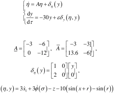
and then the pendulum system with the normal parameters a= =c 10 and b=1 can be written as,

( )

(

)

d

30 ,

d y

A y

y

y y

η

η η δ

εδ η τ

 = +

 

= − +





(22)

where A∈ A A, _,

3 6

0 12

A= − − _ −

 ,

3 3]

13.6 6]

A= − − _ −

 ,

( )

1 0

2 0 0

y y

η

δ

_{= }   _{  }

   ,

(

,

)

31 3

( )

10 sin

(

)

sin

( )

)

y y x z x r r

δ η =  + φ σ − − + − .

By stability theorem of interval matrix [9], it is easy to verify that the interval matrix A is Hurwitz stable. Thus, by solving Lyapunov equation P A_A +A PT _A = −I and P_ΛΛ + ΛTP_Λ = −I, the maximum values of P_A and P_Λ can be obtained, respectively, that is,

0.177

P_η ≤ and P_y ≤0.034. and then using δ ηy

(

,y

)

≤104.5η +14 y and δη

( )

y ≤ 5 y , we have,

1 0.4

β = , β =₂ 1.74 and γ =0.47.

Therefore, the stability of the closed-loop system (22) can be ensured for all ε <0.3 and r∈ −

[

π, π

]

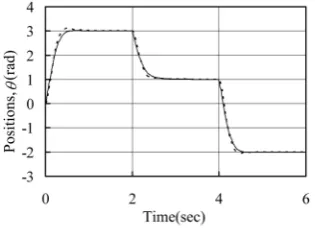
. For illustrating the performance of controller above, the simulations are achieved under normal and perturbed parameters, respectively. The normal parameters are a= =c 10 and b=1. In the perturbed case, b and c

[image:8.595.218.415.246.406.2]

are reduced to 0.25 and 2.5, respectively, corresponding to four times the mass.

Figure 3 showed the simulation results under normal (solid line) and perturbed (dashed line) cases. The fol-lowing observations can be made: the optimum response in the whole domain of interest can all be achieved by a set of the same control gains, even under the case that four times payload changes. This demonstrates that al-though the design method here is too conservative, general integral controller, which is tuned by only the normal parameters, has superstrong robustness, fast convergence, and good flexibility and can deal with nonlinearity and uncertainties of dynamics more forcefully.

5. Conclusions

(9)

[image:9.595.235.393.85.200.2]

Figure 3. System output under normal (solid line) and perturbed case (dashed line).

stabilize the system, just like the system state, such that it does not need to take an extra and special effort to deal with the integral dynamic; 3) No longer resorting to an ordinary control along with a known Lyapunov function, but synthesizing singular perturbation technique, mean value theorem, stability theorem of interval matrix and Lyapunov method, a universal theorem to ensure regionally as well as semi-globally asymptotic sta-bility is established in terms of some bounded information. Consequently, this universal theorem is not sus-pended in midair but is developed with a solid foundation.

Simulation results showed that general integral controller, which is tuned by this design method, has super-strong robustness and can deal with nonlinearity and uncertainties of dynamics more forcefully.

References

[1] Liu, B.S. and Tian, B.L. (2009) General Integral Control. Proceedings of the International Conference on Advanced Computer Control, Singapore, 22-24 January 2009, 136-143.

[2] Liu, B.S. and Tian, B.L. (2012) General Integral Control Design Based on Linear System Theory. Proceedings of the 3rd International Conference on Mechanic Automation and Control Engineering, Baotou, 27-29 July 2012, Vol. 5, 3174-3177.

[3] Liu, B.S. and Tian, B.L. (2012) General Integral Control Design Based on Sliding Mode Technique. Proceedings of the 3rd International Conference on Mechanic Automation and Control Engineering, Baotou, 27-29 July 2012, Vol. 5, 3178-3181.

[4] Liu, B.S., Li, J.H. and Luo, X.Q. (2014) General Integral Control Design via Feedback Linearization. Intelligent Con-trol and Automation, 5, 19-23. http://dx.doi.org/10.4236/ica.2014.51003

[5] Liu, B.S., Luo, X.Q. and Li, J.H. (2013) General Concave Integral Control. Intelligent Control and Automation, 4, 356- 361. http://dx.doi.org/10.4236/ica.2013.44042

[6] Liu, B.S., Luo, X.Q. and Li, J.H. General Convex Integral Control. International Journal of Automation and Compu-ting.

[7] Liu, B.S. (2014) Constructive General Bounded Integral Control. Intelligent Control and Automation, 5, 146-155. http://dx.doi.org/10.4236/ica.2014.53017

[8] Liu, B.S. (2014) On the Generalization of Integrator and Integral Control Action. International Journal of Modern Nonlinear Theory and Application, 3, 4452. http://dx.doi.org/10.4236/ijmnta.2014.32007

[9] Krans, F.J. and Mansour, M. (1991) Sufficient Conditions for Hurwitz and Schar Stability of Interval Matrices. Pro-ceeding of the 30th conference on decision and control, Brighton, December 1991, 3043-3044.

(10)