Munich Personal RePEc Archive
Early Warning System: An Assessment
of Vulnerability
Reinhart, Carmen and Goldstein, Morris and Kaminsky,
Graciela
University of Maryland, College Park, Department of Economics
2000
Early Warning System: An Assesment of Vulnerability
Assessing Financial Vulnerability: An Early Warning System for Emerging Markets Notes from Chapter 5
Morris Goldstein, Graciela L. Kaminsky, and Carmen M. Reinhart (Washington, DC: Institute for International Economics, 2000)
Predicting the timing of currency and banking crises is likely to remain an elusive task
for academics, financial market participants, and policymakers. Few foresaw the Asian crises
and fewer still could have imagined their severity. However, recent events have highlighted the
importance of improving upon a system of “early warnings.” The signals approach introduced in
Kaminsky and Reinhart (1996) and applied to the out-of-sample data during January 1996- June
1997 in this section allows us to glean where trouble spots may be brewing.
Needless to say, such exercises are fraught with the traditional Type I and Type II errors.
Assuming the null hypothesis to be that the economy is in a state of “tranquility,” a high
proportion of indicators flashing leads one to reject that hypothesis in favor of the alternative,
namely that a crisis is likely in the next twenty four months. Yet, a country may be “vulnerable,”
in the sense that a high proportion of variables are signaling trouble, yet the crisis may be averted
through either good luck, good policies, or credible implicit bail-out guarantees. This would be
an example of a Type II error. A recent example of this case is Brazil, in which multiple signals
were flashing as early as 1997 but these warning signs did not culminate into a full-fledged crisis
until 1999. Alternatively, the crisis may occur without much warning signs from the indicators,
this Type I error, or “the dog that did not bark in the night” could be interpreted as evidence of
relevant for understanding the Indonesian crisis.
Vulnerability and signals
Tables 5.1-5.4 summarize some of the key features of applying the signals approach to
the recent data. The first column of the table provides information on the total number of signals
from the 15 monthly indicators listed in Tables 3.1. The second column provides information on
the number of monthly indicators sending signals while the third column lists the number from
the top five indicators, which are real exchange rates, stock prices, the money multiplier, output
and exports for banking crises and real exchange rates, stock prices, exports, M2/reserves, and
output for currency crises. The next three columns give the comparable information for the eight
annual indicators. On the case of the annual indicators, we focus on the top three indicators,
which are short-term capital flows/GDP, current account balance/investment, and the overall
budget deficit/GDP for banking crises; for currency crises the current account deficit/GDP
replaces short-term capital inflows, while the other two indicators are the same. The last column
gives the percent of the twenty three indicators that are signaling. The reason to highlight the
number of top indicators signaling, is that these are the indicators with the lowest noise-to-signal
ratios hence, a signal from these is more meaningful than a signal from a less reliable indicator.
Table 5.1 provides this information for currency crises using the thresholds reported in
Table 3.2. As the last column highlights there is considerable cross-country variation, with the
lowest proportion of signals coming from Egypt and the highest from the Czech Republic, which
enlarged the size of the rejection region by five percent for all the indicators. Hence, for
instance, instead of having a 10 percent threshold for stock prices for the case of currency crises,
we now have a 15 percent threshold. This sensitivity analysis increases the likelihood of having
a Type II error (rejecting the null hypothesis of tranquility when you shouldn’t) while reducing
the probability of a Type I error (not rejecting when you should). In any case, including
“borderline” signals does not alter the picture for some countries (such as Argentina) but it
increases the proportion of indicators signaling markedly, as well as the number of signals, for
countries like Korea (from 48 to 65 percent) and South Africa (from 39 to 52 percent). The next
two tables report the tally for banking crises using the original thresholds (Table 5.3) and the
“borderline” scenario. Not surprisingly, the country profiles that emerge are similar as several of
5.1 Signals of balance of payment crises
Monthly indicators Annual indicators Total
Country Total signals Number of indicators signaling Top indicators signaling Total signals Number of indicators signaling Top indicator s signaling Percent of indicators signaling
Argentina 35 3 1 2 2 0 22
Bolivia 33 6 2 0 0 0 26
Brazil 37 5 3 0 0 0 22
Chile 34 2 1 1 1 0 13
Colombia 27 5 1 3 3 0 35
Czech Republic
77 10 3 4 2 2 52
Denmark 21 3 1 1 1 0 17
Egypt 14 3 2 0 0 0 13
Finland 74 7 1 2 2 0 39
Greece 32 8 2 3 2 0 43
Indonesia 6 3 1 1 1 0 17
Israel 24 4 1 1 1 0 22
Korea 32 8 3 3 3 0 48
Malaysia 36 9 3 0 0 0 39
Mexico 11 2 0 2 2 0 17
Norway 9 3 0 1 1 0 17
Peru 16 2 0 1 1 0 13
Philippines 59 8 1 2 2 0 43
South Africa
42 8 3 1 1 0 39
Spain 44 6 2 1 1 0 30
Sweden 55 5 1 1 1 0 26
Thailand 50 6 3 1 1 1 30
Turkey 22 4 1 3 3 0 30
Uruguay 58 5 0 1 1 0 26
5.2 “Borderline” Signals of balance of payment crises
Monthly indicators Annual indicators Total
Country Total signals Number of indicators signaling Top indicators signaling Total signals Number of indicators signaling Top indicator s signaling Percent of indicators signaling
Argentina 35 3 0 2 2 0 22
Bolivia 33 8 2 0 0 0 35
Brazil 39 7 3 0 0 0 32
Chile 40 5 2 1 1 0 26
Colombia 49 7 3 3 3 0 43
Czech Republic
85 10 3 4 2 2 61
Denmark 28 5 1 2 2 0 30
Egypt 22 3 2 1 1 0 17
Finland 86 8 1 3 2 1 43
Greece 41 8 3 3 3 0 48
Indonesia 9 4 3 1 1 0 22
Israel 37 6 3 1 1 0 30
Korea 63 11 3 5 4 1 65
Malaysia 40 9 3 0 0 0 39
Mexico 24 2 0 2 2 0 17
Norway 31 7 2 1 1 0 35
Peru 26 5 1 2 2 0 30
Philippines 68 8 3 3 3 0 48
South Africa
63 10 3 2 2 0 52
Spain 55 7 2 1 1 0 35
Sweden 60 6 1 1 1 0 30
Thailand 54 6 3 1 1 1 30
Turkey 33 5 3 3 3 0 35
Uruguay 71 5 1 1 1 0 26
5.3 Signals of banking crises
Monthly indicators Annual indicators Total
Country Total signals Number of indicators signaling Top indicators signaling Total signals Number of indicators signaling Top indicator s signaling Percent of indicators signaling
Argentina 36 4 0 1 1 1 22
Bolivia 42 8 2 0 0 0 35
Brazil 39 6 2 0 0 0 26
Chile 34 2 1 1 1 0 13
Colombia 38 5 2 3 3 1 35
Czech Republic
81 10 3 4 2 1 52
Denmark 24 4 0 1 1 0 22
Egypt 18 3 0 0 0 0 13
Finland 77 7 1 3 2 1 39
Greece 39 8 3 2 2 1 43
Indonesia 10 3 2 1 1 1 17
Israel 32 6 3 1 1 0 30
Korea 42 10 4 3 3 1 57
Malaysia 42 9 3 0 0 0 39
Mexico 16 4 1 2 2 0 26
Norway 30 8 2 1 1 0 39
Peru 19 5 1 1 1 0 26
Philippines 59 8 3 2 2 0 43
South Africa
55 10 3 1 1 0 43
Spain 51 7 1 1 1 0 35
Sweden 59 5 1 1 1 0 26
Thailand 53 6 2 1 1 1 30
Turkey 27 5 3 2 2 0 30
Uruguay 74 5 1 1 1 0 26
5.4 “Borderline” signals of banking crises
Monthly indicators Annual indicators Total
Country Total signals Number of indicators signaling Top indicators signaling Total signals Number of indicators signaling Top indicator s signaling Percent of indicators signaling
Argentina 46 7 1 1 1 1 35
Bolivia 45 8 2 0 0 0 35
Brazil 44 9 3 0 0 0 39
Chile 43 7 3 1 1 0 35
Colombia 70 9 3 3 3 1 52
Czech Republic
87 10 3 4 2 2 52
Denmark 29 6 1 1 1 0 30
Egypt 24 3 0 0 0 0 13
Finland 88 8 1 3 2 1 43
Greece 50 9 4 2 2 1 48
Indonesia 14 4 3 1 1 1 22
Israel 49 8 4 1 1 0 39
Korea 74 13 5 3 3 1 61
Malaysia 49 9 3 0 0 0 39
Mexico 30 5 1 2 2 0 30
Norway 37 8 2 1 1 0 39
Peru 27 6 2 1 1 0 30
Philippines 73 8 3 2 2 0 43
South Africa
68 10 3 1 1 0 48
Spain 58 9 2 1 1 0 43
Sweden 66 8 2 1 1 0 39
Thailand 58 9 3 1 1 1 43
Turkey 35 6 3 2 2 0 35
Uruguay 86 6 1 1 1 0 30
So who is vulnerable? Ideally, we want to take into account whether a country is
vulnerable to either a currency or a banking crises, since so often the two go hand-in-hand. One
would also like to give a higher weight to the more reliable indicators. Kaminsky (1998)
constructs such a composite index to gauge the probability of a crisis conditioned on multiple
signals from various indicators; the more reliable indicators receive a higher weight in the
composite index. This methodology and its out-of-sample results are described in the latter part
of this chapter.
While we do not tabulate the probability of a crisis in this exercise (this is take up in the
following part of this chapter), conditioned on a composite index, in what follows, some of the
information on the incidence of signals and the quality of the indicators signaling is presented in
summary form for the twenty “emerging market economies” in our sample for currency and
banking crises in Table 5.5. The first column tallies a count of the “weighted” signals. Each
indicator either sends a signal which we assign the value of one, or does not signal, to which we
assign a value of zero. Yet, simply counting the proportion of indicators signaling (as in Tables
5.1-4) does not discriminate among the highly heterogenous performance of the indicators.
To remedy this, we begin by eliminating from our list of potential leading indicators
those variables which had a noise-to-signal ratio above unity; this is tantamount to stating that
their marginal forecasting ability (P(CS)=0 or less. As Table 3.1 highlights, for banking crises,
this eliminates imports, the lending-deposit ratio, the terms of trade, government consumption
growth, and FDI/GDP. For currency crises, this drops from the list the domestic-foreign interest
rate differential, the lending-deposit ratio, bank deposits, central bank credit to the public sector
and FDI/GDP. For the remaining indicators with noise-to-signal ratios below unity, we weighed
currency crisis let’s suppose that both the real exchange rate and imports are issuing a signal; the
former would receive a weight of 4.55 (or 1/0.22) while the latter would only receive a weight of
1.49 (or 1/0.87). If all 18 remaining indicators were sending signals, the maximum value that
this index could score is 30.05 for banking crises and 33.23 for currency crisis. This score is a
simple sum of the inverse of the noise-to-signal for the indicators that are retained. However, it
is seldom the case that every indicator signals. Table 5.5 presents the composite score of the
indicators that are signaling for 20 of the emerging markets in our sample for currency and
banking crises separately. The first column provides the relevant value for a currency crisis,
while the second provides information on the vulnerability of the country (by this measure)
relative to the remaining 19 countries. Hence, South Africa, the Czech Republic, and Thailand
registered as the most vulnerable on the basis of the signals issued and the quality of those
signals in the January 1996-June 1997 period.
For banking crises, the comparable exercise places the Czech Republic, Korea, and
Greece as the most vulnerable. Perhaps, not surprisingly, near the bottom of the list are countries
such as Mexico and Venezuela which are still recovering from their 1994-95 crises.
Lastly, to assess the extent of vulnerability to financial crises, using alternatives measures
we provide information in Table 5.6 on: i) the average proportion of indicators signaling
banking and currency crises; ii) average proportion of the top eight indicators (monthly and
annual) that are signaling; and the average of the “weighted” indices reported in Table 5.5 for
currency and banking crises. The table also ranks the countries, by these three criteria,
5.5 “Weighing” the signals: Currency and banking crises in emerging markets
Currency crises Banking crises
Country Weighted signals Rank Weighted signals Rank
Argentina 5.41 16 7.98 10
Bolivia 6.59 12 7.30 13
Brazil 7.57 10 6.08 14
Chile 5.90 15 5.74 16
Colombia 10.59 8 11.87 6
Czech Republic*
15.42 2 17.24 1
Egypt 6.02 14 8.33 9
Greece 14.27 6 14.15 3
Indonesia* 7.54 11 8.33 9
Israel 6.30 13 10.38 8
Korea* 14.57 4 14.55 2
Malaysia* 12.46 7 7.74 12
Mexico 2.82 19 2.59 19
Peru 2.82 19 5.33 17
Philippines* 14.40 5 11.52 7
South Africa
16.52 1 12.74 4
Thailand* 14.63 3 12.09 5
Turkey 8.21 9 7.87 11
Uruguay 4.40 18 4.88 18
Venezuela 5.28 17 6.02 15
5.6 The vulnerability to financial crises in emerging markets: Alternative measures
Country Average proportion of
indicators signaling both
crises
Rank Average proportion top nine indicators signaling both
crises
Rank Average of the “weighted”
signals
Rank
Argentina 29 11 11 5 6.69 14
Bolivia 35 8 22 4 6.94 12
Brazil 36 7 33 3 6.82 13
Chile 31 9 33 3 5.74 17
Colombia 48 4 44 2 11.23 7
Czech Republic* 57 2 56 1 16.33 1
Egypt 15 15 11 5 6.42 15
Greece 48 4 44 2 14.21 4
Indonesia* 22 14 44 2 7.93 11
Israel 35 8 44 2 8.34 9
Korea* 63 1 56 1 14.56 3
Malaysia* 39 6 33 3 10.10 8
Peru 30 10 22 4 4.08 19
Philippines* 46 5 33 3 12.96 6
Mexico 24 13 11 5 2.71 20
South Africa 50 3 33 3 14.63 2
Thailand* 35 8 44 2 13.36 5
Turkey 35 8 33 3 8.04 10
Uruguay 28 12 11 5 4.88 18
Venezuela 31 9 22 4 6.02 16
Clustered at the top of the list are several of the countries that have had or are still
undergoing a financial crises; these countries are denoted by an asterisk (*). This suggests a
relatively favorable out-of-sample performance for the “signals” approach. The three measure of
vulnerability provide similar rankings for most of the “extreme” cases, such as the Czech
Republic, Korea, Malaysia, and the Philippines, among the countries that have already had crises
and South Africa, Colombia, and Greece among those that have not. In the case of Greece,
however, there was an orderly devaluation, while in Colombia’s case there was both a
devaluation (in August 1998) as well as serious banking sector difficulties. For countries such as
Thailand and to a lesser degree Indonesia taking into account the “quality” of the indicator
signalling changes the overall ranking considerably.
While this exercise allows us to weigh the relative propensity to crisis across countries at
a point in time, indeed, it is akin to a static snap shot, it does not convey information on the
dynamics of the process. To assess to what extent a country is becoming more or less vulnerable
to crisis over time, one would need a continuum of such snap shots. The analysis in the next
section of this chapter, which maps the composite index described in this section onto the
time-varying probability of a crisis fills this gap and allows us to extend our out-of-sample evaluation
of the signals approach.
A Composite Indicator: Methodology
In Chapters 3 and 4, we examined the likelihood of a country falling prey to a speculative
attack or to a banking crisis by focusing on the information provided by individual indicators.
That is, we assessed the odds of a currency crisis after, for example, an appreciation of the
market. This exercise was useful because it allowed us to discriminate among the types of
indicators that may be useful in anticipating the onset of financial crises. At the same time, as
discussed in the previous section, this focus on individual signs of trouble may result in an partial
picture of an economy in the eve of financial crises. This is because, while currency and banking
crises may arise as a result of an isolated shock, most of the time they are preceded by more
systemic problems in the economy, including the financial sector.1
Most often, crises erupr as the economy collapses under the strain of losses in
competitiveness, a deterioration of the current account, a profound slowdown in growth, burst of
stock bubbles, and the “credit crunches” that typically follow overlending cycles. Thus, we need
to combine these individual manisfestations of problems into an indicator of economic distress
that is continuously evolving.
As discussed earlier, one straightforward way of capturing the fragility of the economy at
the onset of a crisis is to keep track of the number of signals being issued in the different sectors
of the economy. Presumably, the larger the number of red flags coming from different sectors of
the economy, the higher the odds of a financial collapse. However, the number of individual
indicators “signaling” does not fully use the information provided by the univariate indicators
because it does not account for the different forecasting ability of each variable.
To account for ( i) the multiplicity of problems in the economy; (ii) the heterogeneous
forecasting ability of the univariate indicators; and (iii) the time-varying dimension of the
likelihood of a crisis (an issue that we did not address in the previous cross-country
comparisons), we construct the following composite indicator,
In (5.1) it is assumed that there are n different univariate indicators. Each indicator has a
differentiated ability to forecast crises and, as before, this ability can be summarized by the
noise-to-signal ratio, here denoted by j. St jis a dummy variable that is equal to one if the
univariate indicator, S j crosses its critical threshold and is thus signaling a crisis and zero
otherwise. As before, the noise-to-signal ratio is calculated under the assumption that an
indicator issues a correct signal if a crisis occurs within the following 24 months. All other
signals are considered false alarms.
Once we construct this composite indicator, we can then proceed as we did with the
individual indicators in Chapters 2- 3 to choose a critical value for the composite indicator so
that when the composite indicator crosses this threshold, a crisis is deemed to be “imminent.”2
As before, this “critical” threshold could chosen so as to be the one that minimizes the
noise-to-signal ratio of the composite indicator. Moreover, we could also calculate the
probability of a crisis conditional on the composite indicator signaling a crisis (i.e., crossing the
critical threshold) as well as the odds of a crisis when the composite indicator is not signaling.
2 Meaning, as in the individual indicators, in the next 24 months. ωj
t j n
1 j= t= S
/
However, this procedure would not give us an exhaustive report of the extent of the built-up of
weakness in the economy as the crisis approaches. Since, it is dichotomous, it will only provide
two types of information–namely, signal or no signal.
To introduce shades of grey,however, we are going to proceed somewhat differently in
what follows. We are going to track the build-up of weaknesses in the economy and assess the
how the likelihood of a crisis evolves over time. For each value of the composite indicator at a
point in time we will calculate the corresponding probability of a crisis. Hence, as the numerical
value of the composite indicator increases (as the number of reliable signals increase)–so does
the probability of a crisis.
The idea is to analyze the empirical distribution of the indicator jointly with the
occurrences of crises and estimate probabilities of crises conditional on different values of the
composite indicator. We would like to evaluate what the odds of a crisis are if none of the
univariate indicators are signaling, that is when the composite indicator takes on a value of zero
or when all the univariate indicators are signaling and the composite reaches its maximum value.
But we would also like to evaluate the intermediate scenarios, which depend on both how many
and which of the indicators are signaling, as the more reliable indicators are assigned a higher
weight in the composite. For example, we would like to calculate the probability of a crises
conditioned on knowing that the value of the indicator is in the 9-12 range, which as we saw
from the cross- section analysis earlier in this chapter was associated with a number of the recent
crises (see Table 5.5).
In practice, we can construct this set of probabilities using the information on the value of
the composite indicator for all the countries in the sample together with the information on
where I is the lower bound of the range we are interested in (9 in our earlier example) and is
the upper bound of the range we are interested in (12 in our example).
Hence, as before, we have the following two by two matrix,
Crisis occurs in the following 24 months
No crisis occurs in the following 24 months
A B
C D
These probabilities will be estimated using all the information from all the countries in
the sample. Once we estimate these probabilities and using the information on the number of
signals being issued at any moment of time, we can construct time series probabilities of crisis
for every country Ptm is the probability of crisis of country m in period t.
Once we construct these time series of crises probabilities, we can also evaluate the
forecasting ability of the composite indicator and compare its track record to that of other
indicators, such our top-ranked univariate indicator, the real exchange rate. To conduct this
“horserace,” we follow Diebold and Rudebusch (1989) and employ the Quadratic Probability
Score (QPS) as our metric of goodness of fit. In particular, the QPS evaluates the average
closeness of the predicted probabilities and the observed realizations, as measured by a dummy
variable that takes on a value of one when there is a crisis and zero otherwise. 3
3 This approach has been also to assess the ability of various indicators to anticipate turning points in the business cycle (see Diebold and Rudebusch 1989).
B) + A/(A = ) I < I < I |
where k=1,2,3 refers to the indicator, Pkt, refers to the probability associated with that indicator
and Rt are the zero-one realizations. The QPS rages from zero to two, with a score of zero
corresponding to perfect accuracy.
A Composite Indicator: Empirical Results
The methodology described in Chapter 5 was applied to the countries in the sample. In
what follows, we first examine the sample probabilities of crises using the information from the
composite indicator so as to have a reading on the links between the state of the economy and the
eruption of banking and currency crises. Second, we examine the performance of the composite
indicator both in-sample and out-of-sample and we rank the indicator ability relative to that of a
naive forecast of crises and that of the best univariate indicator: the real exchange rate. Third, we
examine the onset of the Asian crisis as captured by the probabilities of crises obtained using the
composite indicator.
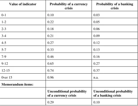
Table 5.7 reports the conditional probabilities of both currency and banking crises using
the composite indicator. The left-hand side panel reports the likelihood of currency crises.
When almost none of the indicators are signaling a future crisis, the composite indicator takes
on values between zero and two, the probability of a currency crisis is about 10 percent, and
substantially smaller than the unconditional probability of crisis, that is about 30 percent.
However, the probability of a currency crisis increases sharply and nonlinearly as the signs of
vulnerability of the economy increase, with the probabilities of a currency crisis reaching almost
100 percent when the indicator is about 15 or larger. The right panel reports the same evidence )
R -P 2( 1/T =
QPS kt t 2
T
for banking crises. As in the case of currency crises, the probabilities of a collapse of the banking
sector increase sharply as the economy deteriorates. However, as we found with the univariate
indicators, banking crises (Chapter 3) are harder to anticipate. Even when nearly
all the univariate indicators are signaling, the probability of a banking crisis only climbs to about
[image:19.612.73.541.293.653.2]40 percent.
Table 5.7 The Composite Indicator and Conditional Probabilities of Financial Crises
Value of indicator Probability of a currency crisis
Probability of a banking crisis
0-1 0.10 0.03
1-2 0.22 0.05
2-3 0.18 0.06
3-4 0.21 0.09
4-5 0.27 0.12
5-7 0.33 0.13
7-9 0.46 0.16
9-12 0.65 0.27
12-15 0.74 0.37
0ver 15 0.96 n.a.
Memorandum items:
Unconditional probability of a currency crisis
Unconditional probability of a banking crisis
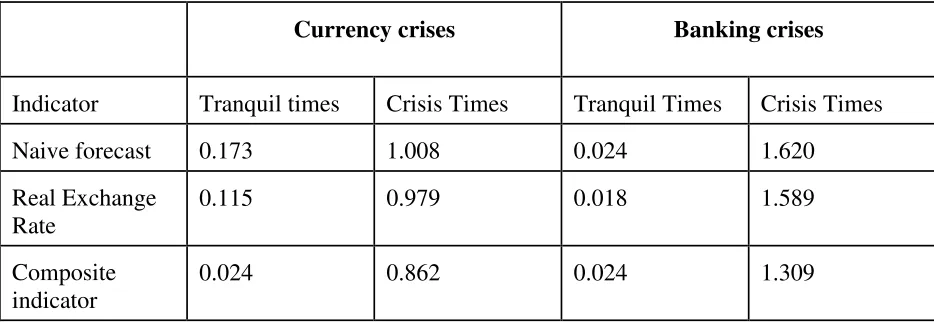
The top panel in Table 5.8 looks at currency crises, the bottom panel examines the same
evidence for banking crises. In both cases, the performance of the composite indicator is
compared to the performance of the real exchange rate--the best univariate indicator-- as well as
the naive forecast based on the unconditional probability of crisis. The score statistics are
reported separately for “Crisis Times” and for “Tranquil Times” to examine whether the
performance of the different leading indicators varies across regimes.
As shown in the top panel, the real exchange makes a substantial improvement over the
unconditional forecast of currency crises, with the forecasting accuracy in tranquil times
increasing substantially more than in crisis times. Overall, the composite indicator performs
better--in terms of accuracy-- than the real exchange rate, but the larger improvements are
obtained when forecasting in crisis times, suggesting that in fact, crises erupt (more often than
not) when there is widespread economic distress.
As shown in the bottom panel, all indicators score worse when predicting the onset of the
banking crises, that is the 24 months around the beginning of the banking crises. As it was
examined before, the real exchange rate makes some improvement over the unconditional
forecast of financial crises in general. For example, the quadratic probability score declines from
0.024 and 1.620 for the naive forecast of currency crises to 0.018 and 1.589 for the real exchange
rate forecast during tranquil and crisis times, respectively. The composite indicator outperforms
the real exchange rate when forecasting the onset of crisis, but is in general outperformed by the
real exchange rate during tranquil times. This is explained by the fact that the real exchange rate
Table 5.8. Scoring the Forecasts: Quadratic Probability Scores
Currency crises Banking crises
Indicator Tranquil times Crisis Times Tranquil Times Crisis Times
Naive forecast 0.173 1.008 0.024 1.620
Real Exchange Rate
0.115 0.979 0.018 1.589
Composite indicator
0.024 0.862 0.024 1.309
A Composite Indicator: An Out-of-Sample Application to Southeast Asia
Using the information on the monthly value of the composite indicator and the
conditional probabilities of crises in Table 5.7, we can construct series of probabilities of crises
for countries both in-sample, from January 1970 to December 1995, and out-of-sample, from
January 1996 to December 1997. As an illustration, Figure 1 reports, the time-series probabilities
of currency crises implicit in the composite indicator for four Southeast Asian economies in the
1990s. The shaded areas in the figures are “crisis times.” Table .. complements this information
by providing desaggregated information on the source of the signals. This table quantifies, crisis
by crisis, the number of the indicators showing “unusual” behavior in the 24-month period prior
these crises, with a 1 denoting unusual behavior and a 0 denoting normal behavior.
With the exception of Indonesia, all the Southeast Asian countries show a severe state of
distress with about 65 percent of the indicators flashing signals. These currency crises are the
enter a marked slowdown in growth after a prolonged boom in economic activity fueled by rapid
credit creation.4 This dramatic surge in credit is, in large part, explained by heavy capital inflows
and partly by the reform of the financial system, which is accompanied by drastic reductions in
reserve requirements. Overall, the explosive growth in these countries comes to an end with a
real appreciation of the domestic currencies (which are, in differing degrees, tied to the U.S.
dollar) and the corresponding loss of export markets. It is noteworthy that during the latter part
of this period there is a substantive appreciation of the dollar vis-a-vis the yen.
For instance, short-term capital inflows to Thailand amount to 7-10 percent of GDP in
each of the years 1994-1996, with the growth rate of credit to the nonfinancial private sector over
1990-1995 amounting to more than 23 percent. While in the early 1990s, output growth rates
increase to almost 9 percent fueled in part by easy credit, this rapid economic growth in Thailand
shows signs of coming to an end with the real appreciation of the domestic currency and the
corresponding loss of exports markets (the annual growth rate of exports falls from a peak of 30
percent per year in 1994 to about 0 in 1996). Financial sector fragilities are also evident, with
runs against major banks starting to occur as early as May 1996. Finally, the sharp increase in
interest rates in 1997 to defend the baht puts the nail in the coffin of the already defunct banking
sector.5 Overall, 75 percent of the indicators for which there is available data were exhibiting
“anomalous” behavior.
4This is at odds with the interpretation of these crises provided in Radelet and Sachs (1998), who argue these crises are the byproduct of a financial panic.
The boom-bust cycle in lending is also evident in the Philippines, fueled as in Thailand
by capital inflows but also by a dramatic reduction in reserve requirements, as they underwent
financial liberalization. Bank credit increases by 44 percent a year in 1995-1996. As in Thailand,
the rapidly expanding credit is an important contributor to the rally in stock and real estate
markets, with a four-fold increase in prices in both markets. As in other countries in the region,
foreign currency exposure increases in the Philippines in the 1990s through foreign borrowing to
finance domestic lending, with foreign borrowing concentrated at short maturities. Consumer
lending also increases and fuels a surge in consumption, leading to a deterioration of the current
account, which is accentuated by the real exchange rate appreciation of the domestic currency.
The loss of competitiveness anticipates a future decline in growth and also contributes to a
substantial deterioration of the quality of banks' assets, further reducing the odds of survival of
many individual financial institutions. Overall, in the Philippines, about 50 percent of the
indicators are signaling the increased vulnerability of the economy in the two years prior to the
collapse of the implicit peg in July 1997.6
Malaysia has a number of features in common with Thailand. It is also affected by the
slowdown in the region, though to a much smaller degree. It also has current account deficits
similar in magnitude to those in Thailand in the period 1990-1995, although in 1996 the outlook
of the external sector improves somewhat with the current account/GDP ratio shrinking to -5.3
6 The Philippines was classified as a managed float in the IMF’s exchange rate
percent (in Thailand the current account/GDP ratio in 1996 is still -8.0 percent). Moreover,
Malaysia as Thailand accumulates debt rapidly in the 1990s, with capital inflows fueling a stock
and real estate market boom, with prices increasing about 300 percent in the early 1990s.
Malaysia is also suffering from financial sector vulnerabilities (although not to the same extent
as the other) as a result of the high degree of leveraging in the economy. Indeed, Malaysia has
one of the highest credit-to-GDP ratio in the world and the banks have a large exposure to the
property and equity markets. For Malaysia, about 60 percent of the indicators are showing signs
of distress at the onset of the crisis.
Indonesia, however, looks somewhat different. While it is still true that, as the other
countries in the area, it is exhibiting banking fragilities and short-term debt sharply exceeds
available foreign exchange reserves (about 1.7 times the stock of foreign exchange reserves of
the country).7 the current account deficit is not deteriorating as fast --only reaching 3.5 percent of
GDP in 1996, the slowdown in growth is not yet evident, and the real exchange rate does not
appreciate as much as in the other countries in the region. Only very few indicators (less than 20
percent) are showing signs of strains in the economy in the months prior to the crisis. While the
degree of distress in the domestic economy in the months prior to the crisis cannot explain the
meltdown of the rupiah and of the economy as a whole in 1998, the flurries of financial crises in
1997 do add a severe element of instability as Indonesia and the other countries in the region are
left scrambling for liquidy when Japanese banks --the major lenders to the region-- pull out
rapidly across countries after the major losses suffered in the wake of the Thai crisis.8
7 The beginning of banking crisis in Indonesia can be dated to November 1992 when a large bank (Bank Summa) collapses and triggers runs on three smaller banks. Most state-owned banks are also experiencing serious difficulties.
$50 billion in 1996 to an outflow of US $21 billion in 1997. See, Kaminsky and Reinhart
This chapter has focused on a specific early warning system for currency crises, which
basically highlights that poor domestic economic conditions, either due to mistakes in public
policy or private sector behavior, are the trigger mechanism of financial crises. We have also
examined, however, that this was not always the case. As we examine in greater detail in the
next chapter, the frailty of an economy can be exacerbated by currency crises in other countries.
For example, Indonesia falls prey of a liquidity crunch when Japanese banks recall their loans
from all the Asian countries they had made loans to after suffering major losses with the
devaluation of the Thai baht. Similarly, the fierce but unsucsseful speculative attack on the
Argentine peso following the devaluation of the Mexican peso are difficult to explain on
exclusively on the basis of economic fundamentals at the time of the attack. In the next chapter,
we combine the information on the domestic economy with that of possible spillover effects
REFERENCES
Agenor, Pierre-Richard, Jagdeep S. Bhandari, and Robert P. Flood. 1992. “Speculative Attacks and Models of Balance of Payments Crises.” IMF Staff Papers 39 (June), 357–94.
Bank of International Settlements. 1998. The Maturity, Sectoral, and Nationality Distribution of International Bank Lending. Basle: Bank for International Settlements.
Berg, Andrew, and Catherine Patillo. 1999. “Are Currency Crises Predictable? A Test.” forthcoming in Journal of International Money ad Finance, (August).
Blanco, Herminio, and Peter M. Garber. 1986. “Recurrent Devaluation and Speculative Attacks on the Mexican Peso.” Journal of Political Economy, 94 (February ), 148–66.
Borensztein, Eduardo, and José de Gregorio. 1998. “Devaluations and Inflation After Currency Crises.” Unpublished paper.
Calomiris, Charles, 1997. The Post Modern Bank Safety Net: Lessons from Developed and Developing Countries. Washington, DC: American Enterprise Institute.
Calvo, Guillermo A. 1998. “Varieties of Capital-Market Crises.” In Guillermo A. Calvo and M. King The Debt Burden and Its Consequences for Monetary Policy. New York:
MacMillan Press.
Calvo, Guillermo A., Morris Goldstein. 1996. “What Role for the Official Sector? “In
Guillermo A. Calvo, Morris Goldstein, and Eduard Hochreiter Private Capital Flows to Emerging Markets After the Mexican Crisis, Washington: Institute for International Economics, 233-82.
Calvo, Guillermo A., and Enrique Mendoza. 1996. “Mexico's Balance-of-Payments Crisis: A Chronicle of A Death Foretold,” Journal of International Economics 41, No. 3/4, (November), 235-264.
Calvo, Sara, and Carmen M. Reinhart. 1996. “Capital Flows to Latin America: Is There
Evidence of Contagion Effects?.” In Guillermo A. Calvo, Morris Goldstein, and Eduard Hochreiter Private Capital Flows to Emerging Markets After the Mexican Crisis, Washington: Institute for International Economics, 151–71.
Ratings,” Federal Reserve Bank of New York Economic Policy Review, (October), 1-15.
Cantor, Richard, and Frank Packer. 1996b. “Sovereign Risk Assessment and Agency Credit Ratings,” European Financial Management, Vol. 2, 247-56.
Caprio, Gerald, Jr. and, Klingebiel, Daniela. 1996a. “Bank Insolvency: Bad Luck, Bad Policy, or Bad Banking?” in Annual World Bank Conference on Development Economics. Washington, DC: The World Bank, 79-104.
.Caprio, Gerald, Jr. and, Klingebiel, Daniela. 1996b. “Bank Insolvency: Cross-country Experiences.” Unpublished paper.
Claessens, Stijn, and Thomas Glaessner. 1997. “Are Financial Sector Weaknesses Undermining the Asian Miracle? Unpublished paper.
Cooper, Richard. 1971. “Currency Devaluation in Developing Countries.” In G. Ranis, Government and Economic Development, New Haven: Yale University Press.
Corsetti, Giancarlo, Paolo Pesenti, and Nouriel Poubini. 1997. "What Caused the Asian Currency and Financial Crisis?". Unpublished paper.
Cumby, Robert, and Sweder van Wijnbergen. 1989. “Financial Policy and Speculative Runs with a Crawling Peg: Argentina 1979–81,” Journal of International Economics 17 (August), 111–27.
Demirguç-Kunt, Asli, and Enrica Detragiache. 1998. “Banking Crises Around the World: Are There Any Common Threads.” IMF Staff Papers, (March).
Diamond, Douglas, and Phillip Dybvig. 1983. “Bank Runs, Liquidity, and Deposit Insurance.” Journal of Political Economy 91 (June), 401-19.
Diebold, Francis and Glen Rudebusch. 1989. “Scoring the Leading Indicators.” Journal of Business 62, No. 3 (July), 369-91.
Dooley, Michael P. 1997. “A Model of Crises in Emerging Markets.” National Bureau of Economic Research Working Paper No. 6300. Cambridge: National Bureau of Economic Research
Doukas, John. 1989. “Contagion Effect on Sovereign Interest Rate Spreads.” Economic Letters 29, 237-41.
Edwards, Sebastian. 1986. “Are Devaluations Contractionary?” Review of Economics and Statistics 68, 501-08.
Edwards, Sebastian. 1989. Real Exchange Rates, Devaluation, and Adjustment: Exchange Rate Policy in Developing Countries. Cambridge, Massachusetts: MIT Press.
Eichengreen, Barry, Andrew Rose, and Charles Wyplosz. 1995. “Exchange Market Mayhem: The Antecedents and Aftermath of Speculative Attacks.” Economic Policy 21 (October), 249–312.
Eichengreen, Barry, Andrew Rose, and Charles Wyplosz. 1996. “Contagious Currency Crises,” National Bureau of Economic Research Working Paper 5681, (July).
Eichengreen, Barry, Andrew Rose. 1997. “Staying Afloat When the Wind Shifts: External Factors and Emerging-Market Banking Crises.” Unpublished paper.
Eschweiler. 1997. Did the Market See the Asian Crisis Coming? Unpublished paper.
Fischer, Stanley. 1993. “The Role of Macroeconomic Factors on Growth,” Journal of Monetary Economics 32 (3), 395-415.
Frankel, Jeffrey A., and Andrew K. Rose. 1996. “Exchange Rate Crises in Emerging Markets.” Journal of International Economics 41, No. 3/4 (November), 351-68.Frankel, Jeffrey A., and Sergio L Schmukler 1996. “Crisis, Contagion, and Country Funds: Effects on East Asia and Latin America.” In Reuven Glick Managing Capital Flows and Exchange Rates: Perspectives from the Pacific Basin. Cambridge: Cambridge University Press. 232-266.
Furman, Jason, and Joseph E. Stiglitz. 1998. “Economic Crises: Evidence and Insights from East Asia.” Forthcoming in Brookings Papers on Economic Activity 2, (June).
Galbis, Vicente. 1993. “High Real Interest Rates Under Financial Liberalization: Is There a Problem?.” International Monetary Fund Working Paper WP/93/7, January.
American Development Bank, 27-63.
Gerlach, Stefan, and Frank Smets. 1994. “Contagious Speculative Attacks.” CEPR Discussion Paper No. 1055, (November), London: Center for Economic Policy Research.
Goldstein, Morris. 1996. “Presumptive Indicators/Early Warning Signals of Vulnerability to Financial Crises in Emerging Market Economies.” Unpublished paper.
Goldstein, Morris. 1997. “The Case for an International Banking Standard.” Policy Analyses in International Economics 47, (April), Washington, DC: Institute for International
Economics.
Goldstein, Morris. 1998a. “Early Warning Indicators and The Asian Financial Crisis” Unpublished paper.
Goldstein, Morris, 1998b. The Asian Financial Crisis: Causes, Cures, and Systemic
Implications.”Policy Analyses in International Economics 55, (June), Washington, DC: Institute for International Economics.
Goldstein, Morris. 1998. “Commentary: The Causes and Propagation of Financial Stability: Lessons for Policy makers. In Federal reserve Bank of Kansas City Maintaining
Financial Stability in a Global Economy. Kansas City: Federal Reserve Bank of Kansas City.
Goldstein, Morris. 1998. “Banking Crises: International Experience. In Gerard Caprio, George Kaufman, and Danny Leipziger Preventing Banking Crises. Chicago: Federal Reserve Bank of Chicago; Washington, DC: The World Bank. Forthcoming.
Goldstein, Morris, and Philip Turner. 1996. “Banking Crises in Emerging Economies: Origins and Policy Options.” Bank for International Settlements Economic Paper No. 46, (October). Basle: Bank for International Settlements.
Goldfajn, Ilan, and Rodrigo O.Valdés. 1995 “Balance of Payments Crises and Capital Flows: The Role of Liquidity.” Unpublished paper.
Honohan, Patrick. 1997. “Banking System Failures in Developing and Transition Countries: Diagnosis and Prediction.” Bank for International Settlements Working Paper No. 39, (January).
International Monetary Fund. 1997a. International Capital Markets, (September). Washington: International Monetary Fund.
International Monetary Fund. 1998a. World Economic Outlook, (May). Washington: International Monetary Fund.
International Monetary Fund. 1998b. International Capital Markets, (September). Washington: International Monetary Fund.
International Monetary Fund. 1998c. World Economic Outlook, (October). Washington: International Monetary Fund.
Kamin, Steven B.. 1988. “Devaluation, External Balance, and Macroeconomic Performance: A Look at the Numbers,” Studies in International Finance, No. 62, (August). Princeton: Princeton University, Department of Economics, International Finance Section.
Kamin, Steven B., and John H. Rogers. 1997. “Output and the Real Exchange Rate in Developing Countries: An Application to Mexico,” Unpublished paper.
Kaminsky, Graciela L. 1998. “Currency and Banking Crises: A Composite Leading Indicator.” International Finance Discussion Paper Series No. 629 (December). Washington: Board of Governors of the Federal Reserve.
Kaminsky, Graciela L., and Carmen M. Reinhart. 1996. “The Twin Crises: The Causes of Banking and Balance-of-Payments Problems,” International Finance Discussion Paper No. 544, (March). Washington: Board of Governors of the Federal Reserve.
Forthcoming in American Economic Review.
Kaminsky, Graciela, and Carmen M. Reinhart. 1998b. “On Crises, Contagion, and Confusion.” Unpublished paper.
Kiguel, Miguel A., and Nita Ghei. 1992. “Devaluation in Low-Inflation Economies,” Policy Research Working Paper 1224. Washington: The World Bank.
Krueger, Anne O. 1978. Liberalization Attempts and Consequences, Cambridge, MA: Ballinger.
Krugman, Paul. 1979. “A Model of Balance of Payments Crises.” Journal of Money, Credit, and Banking 11 (August), 311–25.
Krugman, Paul. 1998. “What Happened to Asia?.” Unpublished paper.
Larraín, Guillermo, Helmut Reisen, and Julia von Maltzan. 1997. “Emerging Market Risk and Sovereign Credit Ratings,” OECD Development Centre Technical Papers No. 124, (April). Paris: The Organisation for Economic Co-operation and Development.
Lee, Suk Hun. 1993. “Are the Credit Ratings Assigned by Bankers Based on the Willingness of Borrowers to Repay?,” Journal of Development Economics 40, (April), 349-59.
Leiderman, Leonardo, and Alfredo Thorne. 1996. In Private Capital Flows to Emerging Markets After the Mexican Crisis, ed. by Guillermo A. Calvo, Morris Goldstein, and Eduard Hochreiter Washington, DC: Institute for International Economics, 1–43.
Lindgren, Carl-Johan, Gillian Garcia, and Matthew Saal. 1996. Bank Soundness and Macroeconomic Policy. Washington, DC: International Monetary Fund.
Lizondo, Saul, and Peter J. Montiel. 1989. “Contractionary Devaluation in Developing Countries: An Analytical Overview.” IMF Staff Papers 36 (March), 182-227.
Mishkin, Frederic S. 1996. “Understanding Financial Crises: A Developing Country Perspective,” in Annual World Bank Conference on Development Economics, Washington, DC: World Bank, 29-62.
Moore, Geoffrey H. 1959. “The 1957-58 Business Contractions: New Model or Old? American Economic Review 49 (May), 292-308.
Morley, Samuel A.1992. “On the Effect of Devaluation During Stabilization Programs in LDCs,” Review of Economics and Statistics 74 No.1 (February), 21-7.
Obstfeld, Maurice, and Kenneth Rogoff. 1995. “The Mirage of Fixed Exchange Rates,” Journal of Economic Perspectives 9, (Fall), 73-96.
Radelet, Steven, and Jeffrey Sachs. 1998. “The East Asian Financial Crisis: Diagnosis, Remedies, Prospects,”Brookings Papers on Economic Activity, 1.
Rojas-Suarez, Liliana. 1998. “Early Warning Indicators of Banking Crises: What Works for Emerging Markets? With Applications to Latin America,” Unpublished paper.
Rojas-Suarez, Liliana, and Steven R. Weisbrod. 1995. Financial Fragilities in Latin America: The 1980s and 1990s. International Monetary Fund Occasional Paper 132, (October). Washington,DC: International Monetary Fund.
Rose, Andrew K., and Lars E.O. Svensson. 1994. “European Exchange Rate Credibility Before the Fall.” European Economic Review 38 (May), 1185-1216.
Sachs, Jeffrey, Aaron Tornell and Andres Velasco. 1996. “Financial Crises in Emerging Markets: The Lessons From 1995.” Brookings Papers on Economic Activity, No. 1, 147–215.
Stock, James H., and Mark W. Watson. 1989. “New Indices of Coincident and Leading Economic Indicators.” NBER Macroeconomics Annual, 351-93.
Valdés, Rodrigo O. 1997. “Emerging Markets Contagion: Evidence and Theory.” Unpublished paper.
Velasco, Andres. 1987. “Financial and Balance of Payments Crises: A Simple Model of the Southern Cone Experience.” Journal of Development Economics 27 (October ), 263–83.
Wolf, Holger C. 1997. “Regional Contagion Effects in Emerging Markets.” Princeton University Working Papers in International Finance, G-97-03, (October).
APPENDIX A: DATA AND DEFINITIONS
Crisis index: The index is a weighted average of exchange rate and reserve changes, with
weights such that the two components of the index have equal conditional volatilities. Since
changes in the exchange rate enter with a positive weight and changes in reserves have a
negative weight attached, readings of this index that were three standard deviations or more
above the mean were cataloged as crises. For countries in the sample that had hyperinflation,
the construction of the index was modified. While a 100 percent devaluation may be traumatic
for a country with low-to-moderate inflation, a devaluation of that magnitude is commonplace
during hyperinflations. A single index for the countries that had hyperinflation episodes would
miss sizable devaluations and reserve losses in the moderate inflation periods, since the historic
mean is distorted by the high-inflation episode. To avoid this, we divided the sample according
to whether inflation in the previous six months was higher than 150 percent and then
constructed an index for each subsample. Our cataloging of crises for these countries coincides
fairly tightly with our chronology of currency market disruptions. Eichengreen, Rose, and
Wyplosz (1995) also include interest rates in this index, however, our data on
market-determined interest rates for developing countries does not span the entire sample.
The indicators:
Sources: International Financial Statistics (IFS), International Monetary Fund; Emerging
Market Indicators, International Finance Corporation (IFC); World Development Indicators, the
World Bank, when data was missing from these sources, central bank bulletins and other
country-specific sources were used as supplements. Unless otherwise noted, we used 12-month
2. Domestic credit/nominal GDP: IFS line 52 divided by IFS line 99b (interpolated). Monthly
nominal GDP was interpolated from annual or quarterly data.
3. Real interest rates on deposits: IFS line 60l, monthly rates, deflated using consumer prices
(IFS line 64) expressed in percentage points.
4. The ratio of lending rates to deposit rates: IFS line 60p divided by IFS line60l; was used in
lieu of differentials to ameliorate the distortions caused by the large percentage point spreads
observed during high inflation. In levels.
5. “Excess” real balances: M1 (IFS line34) deflated by consumer prices (IFS line 64) less an
estimated demand for money. The demand for real balances is determined by real GDP
(interpolated IFS line99b), domestic consumer price inflation, and a time trend. Domestic
inflation was used in lieu of nominal interest rates, as market-determined interest rates were not
available during the entire sample for a number of countries; the time trend (which can enter
log-linearly, linearly, or exponentially) is motivated by its role as a proxy for financial
innovation and/or currency substitution. Excess money supply (demand) during pre-crisis
periods (mc) is reported as a percent relative to excess supply (demand) during tranquil times
(mt)--that is, 100 x (mc-mt)/mt.
6. M2 (in US dollars)/reserves (in US dollars): IFS lines 34 plus 35 converted into dollars
(using IFS line ae) divided by IFS line 1L.d.
7. Bank deposits: IFS line 24 plus 25.
8. Exports (in US dollars): IFS line 70.
9. Imports (in US dollars): IFS line 71.
(IFS line 75). For those developing countries where import unit values (or import price indices)
were not available, an index of prices of manufactured exports from industrial countries to
developing countries was used.
11. The real exchange rate: This measure used is based on consumer price indexes (IFS lines
64) and is defined as the relative price of foreign goods (in domestic currency) to the price of
domestic goods. If the central bank of the home country pegs the currency to the dollar
(Deutsche mark), the relevant foreign price index is that of the United States (Germany). Hence,
for all the European countries the foreign price index is that of Germany while for all the other
countries, consumer prices in the United States were used. The trend was specified as,
alternatively, log-linear, linear, and exponential; the best fit among these was selected on a
country-by-country basis. Deviations from trend during crisis periods (dc) were compared to
the deviations during tranquil times (dt) and are shown in Figures 2 and 3 as a percent of the
deviations in tranquil times (i.e.,100 x (dc-dt)/dt).
12. Reserves: IFS line 1L.d.
13. Domestic-foreign interest rate differential on deposits: Monthly rates in percentage
points. IFS lines 60l. Interest rates in the home country are compared with interest rates in the
United States (Germany) if the domestic central bank pegs the currency to the dollar (Deutsche
14. Output: For most countries, the measure of output used is industrial production (IFS
line 66). However, for some countries (the commodity exporters) an index of output of
primary commodities is used (IFS lines 66aa).
15: Stock returns (in dollars): IFC global indices are used for all emerging markets; for
industrial countries the quotes from the main bourses are used.