A New Unsupervised Clustering based Feature Extraction Method

(1)

A new Unsupervised Clustering-based Feature

Extraction Method

Sabra El Ferchichi

LACS

National School of Engineering at Tunis, Tunisia

Salah Zidi

LAGIS

Lille University of Science and Technology, France

Kaouther Laabidi

LACS

National School of Engineering at Tunis, Tunisia

ABSTRACT

In manipulating data such as in supervised or unsupervised learning, we need to extract new features from the original features for the purpose of reducing the dimension of feature space and achieving better performance. In this paper, we investigate a novel schema for unsupervised feature extraction for classification problems. We based our method on clustering to achieve feature extraction. A new similarity measure based on trend analysis is devised to identify redundant information in the data. Clustering is then performed on the feature space. Once groups of similar features are formed, linear transformation is realized to extract a new set of features. The simulation results on classification problems for experimental data sets from UCI machine learning repository and face recognition problem show that the proposed method is effective in almost cases when compared to conventional unsupervised methods like PCA and ICA.

General Terms

Pattern Recognition, Machine Learning, Feature Extraction, and Data mining.

Keywords

Unsupervised feature extraction, similarity measure, clustering, face recognition and classification problems.

1. INTRODUCTION

Feature extraction is an important step in data analysis. It can be used as a preprocessor for applications including visualization, classification, detection, and verification. Herein, we are interested in applying feature extraction to classification problems and in particular for face recognition problem. Actually, as the amount of collected data becomes larger, extracting the right features becomes necessary for an efficient classification process. However, when designing a classification system, prior knowledge about effective features in classification processing, are usually unknown. Although the classification performance is a non-decreasing function of the number of features, using a large number of features can be wasteful of both computational and memory resources [1]. In addition, training a classifier with a large number of features describing a finite amount of data can, eventually, degrade the classifier accuracy [2].

Two different approaches exist to address this issue: feature selection which consists on selecting only relevant attributes through a pre-defined criterion for feature’ relevance [3]; and feature extraction which applies a linear or nonlinear transformations to the original set of features to construct new ones [4]. In fact, different Feature Selection strategies lead either to a combinatorial problem or suboptimal solution [4]. For this very reason, finding a transformation to lower

dimensions might be easier than selecting features, given an appropriate objective function. According to whether the class labels are used, Feature Extraction methods can be divided into supervised and unsupervised ones. When labeled data are sufficient, supervised feature extraction methods usually outperforms unsupervised feature extraction methods [5]. However, in many cases obtaining class label is expensive and the amount of labeled training data is often very limited, supervised feature extraction methods may fail on such small labeled-sample problem.

In this work, we are rather interested in unsupervised feature extraction, where no prior knowledge about pdfs of data or about its class-distribution is available. It has been reported through some experiments that the performance of the classifier system can be deteriorated as new irrelevant features are added [7]. This problem can be avoided by extracting new features containing the maximal information about the data. One well known unsupervised feature extraction method is Principal Component Analysis (PCA) [6]. It is derived from eigenvectors corresponding to the largest eigenvalues of the covariance matrix for data. PCA seeks to optimally represent the data in terms of minimal mean square error between the representation and the original data. The main drawback of this method is that the extracted features are not invariant under transformation. Merely scaling the attributes changes the resulting features [7]. However, it may be useful in reducing noise in the data by separating signal and noise subspace. Another unsupervised method Independent Component Analysis (ICA), has been proposed as a tool to find interesting projections of the data [7]. It has been devised for blind source separation problems, and has demonstrated a lot of potential in various applications. It produces statistically independent components based on negentropy (divergence to a Gaussian density function) maximization.

(2)

contact energy of the amino acid and the position in the sequence for the prediction of HIV protease resistance to drugs.

Hence, this work aims to develop a new method which investigates the use of a new similarity-based clustering technique, to perform unsupervised feature extraction for pattern classification problems and face recognition in particular. The new similarity measure that we propose in this work has more general capabilities than the ones discussed above. Actually, in high dimensional data there are many features that have similar tendencies all along the instances of the data set: they describe similar variations of monotonicity (increasing or decreasing). Thus, these features may give related or the same discriminative information for the learning process. This makes such features redundant and useless. Analyzing variations of monotonicity of each feature along the data set can lead us to determine a form of redundancy between features. By using trend analysis, each feature will be totally described by its signature which is statistically distinguished from random behavior. Intuitively, once groups of similar features have been settled, feature extraction can be realized. A linear transformation is applied on each identified cluster of similar features.

The rest of this paper is organized as follows: in section 2, we introduce the new unsupervised method to extract features based on analyzing their tendencies along the data set. A clustering technique based on a new measure of similarity between features is used to identify and gather similar features. In section 3, performance of the proposed Feature Extraction Method based on Clustering (FEMC) is assessed through classification problem and face recognition task. We compare our method to conventional linear unsupervised method PCA and ICA. In section 4, we offer some conclusions and suggestions for future work.

2. FEATURE EXTRACTION METHOD

BASED CLUSTERING

In this section, we introduce our new unsupervised feature extraction method based on clustering (FEMC) for pattern classification problems.

In fact, redundant information is an intrinsic characteristic of high dimensional data which may complicate learning task and degrade classifier performance [7]. Hence, identifying redundant features in data can lead to reduce the dimension without loss of some important information. Existing feature selection solutions use a filter method to select relevant features and eliminate totally redundant features. Although redundant information is not necessarily relevant for establishing discriminating rules of classification, but it has an underlying interaction with the rest of features. Eliminating them totally from feature space may lead to eliminate some predictive information of the inherent structure of data and thereby induce a less accurate classifier. Our goal is then to identify and then transform this form of redundancy in a way that conserves inherent structure of data, and minimizes the amount of predictive information lost.

Intuitively, similar features describe very similar or mostly the same variations of monotonicity along the data set. They might incorporate the same discriminating information. Identifying this form of similarity, through an appropriate metric, grouping them into different clusters and applying a linear transform on each group, are the different steps of our feature extraction approach. Hence, we based our method on clustering algorithm based a new similarity measure to

identify linear or complex relations that would exist between features. Clustering is supposed to discover inherent structure of data [11-12]. It is a method to creating groups of objects, or clusters, in such a way similar objects are grouped together while those that are different are segregated in their distinct samples but to approximate the true partition of the function

Q.The new similarity measure used in feature clustering is devised based on trend analysis of each feature vector along the data set.

2.1 Problem Formulation

A feature extraction process transforms, linearly or nonlinearly, a set of original features into new ones. The new features are supposed to describe completely the instances of a database and to be useful either supervised or unsupervised classification task.

Merely, considering a set of L D-dimensional data



1, 2,....



D L

x x x  , a feature extraction process tries to find a transformationT to apply, such that:

y_iT x

 

_i ;1 i L. (1) The transformed sample d D

i

y  is composed of d D new features ₁, ₂,.... L

d

v v v  . Each feature vectorviis

constituted by the different values corresponding to each instance or sample

1j L

x_{ } . A new metric is devised to characterize similarity between features and a clustering algorithm is applied on the feature space ₁, ,....₂ L

d

v v v  to gather similar features. The new similarity measure formulation used to characterize similarity between features, is inspired from trend analysis. It will be explained in the next section. Hence, the objective function Q to be optimized by the clustering procedure can be defined by:

Q

 

Lj₁ di₁dij, (2) The distance dij between two feature vector viandvj has to

be appropriately defined to get to an optimum result. Hence, clustering process finds similar features and form dclusters whered D, represented each by its centroid:

gkf S

 

k , (3) Where, S_kis the set of n_kfeature vectors

k

s S

v_ belonging to the clusterC_kand the transformationf is defined by:

 

1 1

.

k

n L

k i s

i s

f S w v

 





(4)

Finally, the obtained set of centroids

 

gk is the set of the d

new features that will re-describe the data set



1, 2,....



D L

x x x  .

2.2 Similarity Measure

(3)

distance like Euclidean distance used normally in clustering algorithm is not suitable for our objective. Using Euclidean distance may lead to erroneous results since it computes the mean of difference between each value of two vectors without use of tendency information about them. In fact, two features may have the same mean (or closer means) but they differ completely in their trend.

To describe the monotonicity of each feature vector, we used trend analysis. Actually, a trend is semi-quantitative information, describing the evolution of the qualitative state of a variable, in a time interval, using a set of symbols such as {Increasing, Decreasing, Steady}[13]. In our case, the trend describes the evolution of each feature in a finite set of samples. We proceed by computing the corresponding first order derivative of a feature vector

v

at each point or sample

x

:

1 1

.

i i

dv v v

dx x x



 



(5)

Then, we determine the sign of the derivative in each point by (6). A feature vector L

v is then being represented as an L-dimensional vector composed of a new set of L variables



1, 1,0



  . Distance function devised to compare two feature vectors relies on verifying difference in the sign of tendency between two feature vectors.













0

1

0 sgn 1 .

0 0

dv

dx _decrease

dv dv

f then increase

dx dx

steady dv

dx



 _

 _

 _{ }  _

 _ _ 

 



 _

 

_ifor the learning data set. In fact, in this work we have computed the occurrence of

the pair of variables

  

  , 10,11,1 1, 10, 11, 1 1,00,01,0 1     



in each vector

i

vinstead of computing only the probability of the single variable 



1, 1,0



. A similarity matrix D between all features vectors is then generated such that

 

, 



_i, _j



; , 1... D i j d v v i j n.

2.3 Feature Extraction Schema

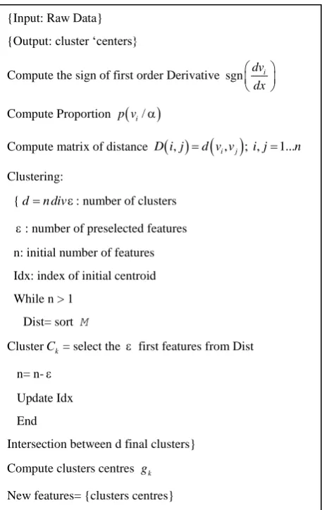
Feature extraction algorithm that we propose in this work, is given by the Figure 1. Clustering algorithm based on the similarity measure described below, is used to form clusters of similar features. It consists at a first step on computing the similarity matrix M between each one of the feature set, based on the metric defined previously by (7). The second step is to perform clustering strategy which is based on C-means clustering. We fix the number of clusters, which correspond indirectly to the number of new extracted features such that:d



n div



,where the threshold  is chosen empirically. Initially, clusters are initialized randomly. Then each clusterCkis formed sequentially by selecting thefirst

ranked features in the similarity matrixM.

They correspond to the set of the most similar features to the corresponding centroidgj. The cluster center is then updated

by computing the new centroid:

gj_{ }1..d W Vj j, (10)

where j 1 j

W I

n is the transform matrix applied to the set of features V_jof the cluster j. n_jis the cardinality of the cluster

j

C and Vjis the matrix containing the features vectors inCj.

Hence, as this process allows an overlap between clusters, since features could be assigned to more than one cluster, we identify common feature between each pair of the obtained clusters. Each common feature is then assigned to the closest cluster according to the Euclidean distance:

 vi



Ck1Ck2



, viCharg min gj_k k1, 2_vi 2.

(11)

(4)

[image:4.595.57.286.69.431.2]

Fig 1: Pseudo-code for FECM algorithm

3. EXPERIMENTAL RESULTS

First, we have conducted the proposed extraction method (FECM) for some well known and largely used data sets from UCI machine learning repository [15]. Second, we have achieved experiments on the face recognition problem through Yale and ORL databases.

3.1 Results on UCI Databases

We have used 4 datasets: Sonar, Pima, Breast cancer and Ionosphere. Some characteristics of these data sets are shown in the Table 1. We have conducted conventional unsupervised feature extraction method PCA and ICA on these data sets and have compared their classification performances with our proposed method FECM for different number of extracted features. We have used Support Vector Machines SVM [16], as a classifier. No pre-treatment has been done for these bases before conducting feature extraction on them.

For SVM, we have used Matlab Toolbox to implement it. The kernel function used is Gaussian kernel and  is set after various tests on 10, 1 or 0.01.

Table 1. Data sets information

Data sets No. of

features

No. of instances

No. of classes

Initial classification

accuracy

Sonar 60 208 2 82.7

Pima 8 768 2 78.0

Breast

cancer 9 569 2

96.6

Ionosphere 34 351 2 91.73

A 13-fold cross validation schema has been used for the sonar data set and 10-fold cross validation was used for the others as in the ref [7].

3.1.1 Sonar data set

[image:4.595.312.571.74.187.2]

This data set was constructed to discriminate between the sonar returns bounced off a metal cylinder and those bounced off a rock. It consists of 208 instances, with 60 features and two output classes: mine and rock. In our experiment, we used 13-fold cross validation in getting the performances as follows: the 208 instances are randomly divided into 13 sets with 16 instances in each.

Fig 2: Classification accuracy on Sonar Data set

For each experiment, 12 of these sets are used as training data, while the 13th is reserved for validation. The experiment is repeated 13 times so that every case appears once as part of a test set. For SVM parameters, we have set  to 1. The Figure 2 shows classification accuracy for different number of extracted features. We can see that the performances of FECM are far better than PCA and ICA except for the case of a very low dimension case of only one extracted feature where ICA outperforms. Since the concept of our approach is to form groups of similar features; extracting a very low number of features means gathering all features in a few numbers of clusters. That can be delicate for some data sets as in this data set. In This case, FECM isn’t the most effective method, nevertheless it still have better classification accuracy than PCA and better than ICA for higher dimension. We can note also that in the case of dimension 9 and 12, FECM is beyond the initial error rate of 82% which is far better than ICA and PCA.

3.1.2 Pima Indian Diabetes data set

It consists of 768 instances in which 500 are class 0 and the others are class 1. It has eight numeric features with no missing value. It has numerous invalid data points, e.g., features that have a value of 0 even though a value of 0 is not meaningful or physically possible. These correspond to points in feature space that are statistically distant from the mean calculated {Input: Raw Data}

{Output: cluster ‘centers}

Compute the sign of first order Derivative sgn dvi

dx

 

 

 

Compute Proportion p v



_i/



Compute matrix of distance D i j

 

, d v v



_i, _j



; ,i j1...n Clustering:

{dn div: number of clusters : number of preselected features

n: initial number of features

Idx: index of initial centroid

While n > 1

Dist= sort M

ClusterCk= select the  first features from Dist

n= n-

Update Idx

End

Intersection between d final clusters}

Compute clusters centres gk

[image:4.595.322.542.315.479.2]

(5)

[image:5.595.325.543.74.234.2]

using the remaining data (with the points in question removed). We removed the points in question from the data set. We have applied PCA, ICA and FECM and compared their performances as we have done for Sonar data set. In training, we have used SVM and the parameter  was set to 10. A 10-fold cross validation has been used for validation process. In following Figure 3, classification performances are presented. We can note that the performances of PCA and ICA get closer as the number of extracted features becomes larger. In this data set, ICA outperforms both PCA and FECM for different numbers of features especially for the lower ones such as dimension 1 and 2.

Fig 3: Classification accuracy on Pima Data set

The proposed method FECM still perform better than PCA and approaches the performances of ICA for higher dimension such as 3 and 5.

3.1.3 Wisconsin Breast cancer data set

This data set consists of nine attributes and two classes; which are benign and malignant. It contains 699 instances with 458 benign and 241 malignant. There are 16 missing values and we replaced these with average values of corresponding attributes as in ref [7]. We compared classification performance of our proposed method FECM with those of ICA and PCA for different number of extracted features. Results are shown in the Figure 4.

We have used a 10-fold cross validation as a strategy of verification. For the SVM classifier, the parameter  was set to 0.01 after we have conducted various experiments. The results show that, with only one extracted feature, FECM can get the maximum classification performance. Hence, for lager number of extracted features, PCA outperform both ICA and FECM.

3.1.4 Ionosphere data set

[image:5.595.62.284.199.361.2]

This radar data was collected by a system in Goose Bay, Labrador. This system consists of a phased array of 16 high-frequency antennas. Received signals were processed using an autocorrelation function whose arguments are the time of a pulse and the pulse number. Instances in this database are described by 2 attributes per pulse number, corresponding to the complex values returned by the function resulting from the complex electromagnetic signal. We compared classification performance of our proposed method FECM with those of ICA and PCA for different number of extracted features. Results are shown in the Figure 5.

Fig 4: Classification accuracy on Breast cancer Data set

[image:5.595.322.542.339.500.2]

We have used a 10-fold cross validation as a strategy of verification. For the SVM classifier, the parameter sigma was set to 10 after we have conducted various experiments. The results show that, with only one extracted feature, FECM can largely outperform ICA and PCA. Hence, for lager number of extracted features, FECM gets either similar or better performance and achieve the best accuracy with 12 features.

Fig 5: Classification accuracy on Ionosphere Data set

3.2 Results on Face Recognition Problem

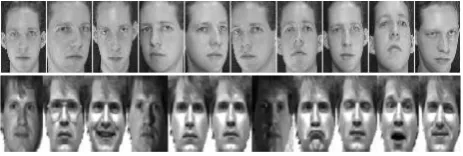
We have used two datasets: Yale and ORL data sets from UCI machine learning repository [15]. The Figure 6 shows some samples from Yale and ORL data sets respectively.

3.2.1 Yale database

It contains 165 GIF images of 15 subjects (subject01, subject02, etc.). There are 11 images per subject, one for each of the following facial expressions or configurations: center-light, w/glasses, happy, left-center-light, w/no glasses, normal, right-light, sad, sleepy, surprised, and wink. The size of each image is 320 x 243, composed of 77760 pixels. In fact, there are many methods to determine the features of the image.

[image:5.595.316.548.664.742.2]

(6)

The most intuitive way is to use each pixel as one feature. The input space becomes too large to be handled. To overcome this constraint we had to accept the loss of some information. Each image was resized to get 783 pixels. The classification performances of extracted features from PCA, ICA and FECM methods were obtained by the leave-one-out schema. The number of extracted features by ICA is the same as that of PCA (PCA is used as a pre-processor for ICA). In the experiments, PCA was initially conducted on 784 pixels and the first 30 PCs were used. The ICA was applied to these 30 PCs. Table 2 shows the classification error rates corresponding to each of these methods. The recognition was performed using the K nearest neighbor classifier (KNN). PCA and ICA produce the same number of features which is 30, but ICA is slightly better than PCA in classification accuracy. It can be seen that our proposed approach outperforms PCA and ICA using only 14 features.

Table 2. Classification performance on Yale Data set

Methods Error rate (%)

(KNN)

No. of features

PCA 24.85 30

ICA 23.03 30

FECM _21.00 14

KNN _21.82 ₇₈₃

3.2.2 ORL database

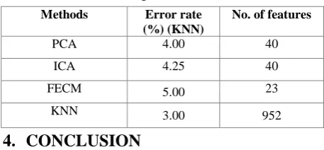
[image:6.595.52.281.488.594.2]

The AT&T database of faces consists of 400 images, which are 10 different images for 40 distinct individuals. It includes various lighting conditions, facial expressions and facial details. The images were cropped into get 952 pixels for computational efficiency. The experiments were performed exactly the same way as in the Yale database. The results in the Table 3 are from the leave-one-out test with the one nearest neighbor classifier. The first 40 PCs are retained as input for ICA. PCA and ICA produces similar results. Our approach is close to PCA and ICA in terms of classification accuracy with smaller number of features which is 23.

Table 3. Classification performance on ORL Data set

Methods Error rate

(%) (KNN)

No. of features

PCA 4.00 40

ICA 4.25 40

FECM _5.00 23

KNN _3.00 ₉₅₂

4. CONCLUSION

This work focuses on developing a general feature extraction approach based on clustering technique for pattern classification task and face recognition in particular. The main motivation behind it was to identify redundancy in feature space and reduce its effect without losing some important information for classification process. Similar feature are recognized through analyzing their tendencies along the data set. Although, trend analysis was used to devise the new similarity measure, it conserves its independency from the order of samples. In the first stage, the proposed approach FECM extracts feature-clusters as features by applying clustering technique, based on the new similarity measure. In the second stage, these features are used for the classification of patterns.

Results obtained from experiments conducted on several data sets, obtained from UCI machine learning repository, showed that this representation of patterns improves over PCA and

ICA in almost of cases, especially when projecting to low dimensions. Except for Pima data set, FECM was not able to improve over other methods in lower dimension, but gets to similar results in higher dimensional projections. For the face recognition task, FECM gets to the lowest dimension with the best accuracy for Yale data set. In the case of ORL data set, FECM gets the lowest dimension with a lower accuracy of 1%.

The transformation applied to the obtained clusters was a linear combination with equal weight applied to each of its corresponding component. However, the transformation we have to apply is a very important step since it has to determine a representative feature of each group. It has to preserve the main characterizes of each group of features and incorporate them into the new representative feature. Thus, an appropriate transformation has to be defined in further work. It would be based on a sophisticated statistical measure of dependency such as Mutual information. In addition, it would be interesting to incorporate label information in the FECM approach for semi-supervised or supervised learning tasks.

5. REFERENCES

[1] Hild II K. E., Erdogmus D., Torkkola K. and Principe J. C. 2006. Feature extraction using information-theoretic learning. IEEE Trans. on pattern analysis and machine intelligence, 28 (September 2006), 1385-1391.

[2] Ripley B.D, Pattern recognition and neural networks. In Cambrigde Univ. Press 1995.

[3] Guyon I., Elisseeff A. 2003. An introduction to variable and feature selection. J. Mach. Learn. 3(March 2003), 1157-1182.

[4] Torkkola K. 2003. Feature extraction by non-parametric mutual information maximization. J. Mach. Learn. 3 (2003), 1415-1438.

[5] Liu X., Tang J., Liu J., Feng Z., "A semi-supervised relief based feature extraction algorithm", in second international conference on future generation communication and networking symposia, 2008.

[6] Saul L. K., Weinberger K. Q., Sha F., Ham J. and Lee D. D. Spectral Methods for Dimensionality Reduction. in O. Chapelle, B. Schoelkopf, and A. Zien (eds.), Semi supervised Learning, MIT Press. Cambridge, MA 2006.

[7] Kwak N. and Chong-Ho C. 2003. "Feature extraction based on ICA for binary classification problems". IEEE Trans. on knowledge and data engineering, 15 (November 2003), 1387-1388.

[8] S. Noam and T. Naftali 2001. "The power of word clusters for text classification", 23rd European colloquium on information retrieval research.

[9] Baker, L. D. and McCallum A. K., 1998. "Distributional clustering of words for text classification", 21st Annual international ACM SIGIR conference on research and development in information retrieval.

[10]Bonet I., Sayeys Yvan, Grau Abalo R., Garcia M.M, Sanchez R., and Van de Peer Y. 2006. Feature extraction using clustering of protein. In proceedings of the 11th Iberoamerican congress in pattern recognition CIARP, 614-623.

[11]Fern X.Z., Brodeley C.E. 2004 Cluster Ensembles for High Dimensional Clustering: an empirical study. Technical report CS06-30-02.

(7)

[13]Charbonier S. and Gentil S 2007. A trend-based alarm system to improve patient monitoring in intensive care units, in Control engineering practice, 15, 1039-1050.

[14]Payne T.R. and Edwards P. 1998. "Implicit feature selection with the value difference metric". 13th

European conference on artificial intelligence, pp.450-454.

[15]http://archive.ics.uci.edu/ml/.