Shuffled Frog Leaping Algorithm based Voltage Stability Limit Improvement and Loss Minimization Incorporating FACTS Devices under Stressed Conditions

Shuffled Frog Leaping Algorithm based Voltage Stability

Limit Improvement and Loss Minimization Incorporating

FACTS Devices under Stressed Conditions

L.Jebaraj C.Christober Asir Rajan S.Sakthivel

V.R.S. College of Engg. and Tech. Pondicherry Engineering College V.R.S. College of Engg. and Tech. Villupuram, Tamil Nadu, India Pillaichavady, Puducherry, India Villupuram, Tamil Nadu, India

ABSTRACT

Recent day power system networks are having high risks of voltage instability problems and several network blackouts have been reported. This phenomenon tends to occur from lack of reactive power supports under heavily stressed operating conditions caused by increased load demand and the fast developing deregulation of power systems across the world. This paper proposes an application of Shuffled Frog Leaping Algorithm (SFLA) based extended voltage stability margin and minimization of loss by incorporating TCSC and SVC (variable susceptance model) devices. The line stability index (LQP) is used to assess the voltage stability of a power system. The location and size of Series connected and Shunt connected FACTS devices are optimized by shuffled frog leaping algorithm. The results are obtained from the IEEE-30 bus test case system under critical loading and single line outage contingency conditions

Keywords

Shuffled Frog Leaping Algorithm, FACTS devices, Line stability index, TCSC, Voltage Stability, SVC.

1.

INTRODUCTION

Present day power system are undergoing numerous changes and becoming more complex from operation, control and stability maintenance standpoints when they meet sudden increasing load demand [1]. Voltage stability is concerned with the ability of a power system to maintain acceptable voltage values at all buses in the system under normal conditions and after being subjected to a critical conditions. A system enters a state of voltage instability when a disturbance, increase in load demand, or change in system condition causes a progressive and uncontrollable decline in voltage level. The main factor causing voltage instability is the inability of the power system to meet the demand for reactive power [2]-[4]. Excessive voltage decline can occur following some severe system contingencies and this situation could be aggravated, possibly leading to voltage collapse, by further tripping of more transmission facilities, var sources or generating units due to overloading. Many large interconnected power systems are increasingly experiencing abnormally high or low voltages or voltage collapse. Abnormal voltages and voltage collapse pose a primary threat to power system stability, security and reliability. Moreover, with the fast development of restructuring, the problem of voltage stability has become a major concern in deregulated power systems. To maintain security of such systems, it is desirable to plan suitable measures to improve power system security and enhance voltage stability margins. [5]-[7].Voltage instability isoneof the phenomena which have result in majorblackouts

.

Recently, several network blackouts have been related to voltage collapses [8].

The Flexible AC Transmission System (FACTS) controllers are capable of supplying or absorption of reactive power at faster rates. The introduction of Flexible AC Transmission System (FACTS) controllers are increasingly used to provide voltage and power flow controls. Insertion of FACTS devices is found to be highly effective in preventing voltage instability [9].Series and shunt compensating devices are used to enhance the Static voltage stability margin.

Voltage stability assessment with appropriate representations of FACTS devices are investigated and compared under base case of study [10]-[12]. One of the shortcomings of those methods is they consider the normal state of the system. However voltage collapses are mostly initiated by a disturbance like line outages. Voltage stability limit improvement needs to be addressed during network contingencies. So to locate FACTS devices consideration of contingency conditions is more important than consideration of normal state of system and some approaches are proposed to locate of facts devices with considerations of contingencies too[13].

Line stability indices provide important information about the proximity of the system to voltage instability and can be used to identify the weakest bus as well the critical line with respect to the bus of the system [14]. A.Mohmed et al is made the derivation of line stability index (LQP) used for stability assessment [15]. From the family of evolutionary computation, Shuffled Frog Leaping Algorithm (SFLA) is used to solve a problem of real power loss minimization and Voltage stability maximization of the system.

The SFLA is a meta-heuristic optimization method which is based on observing, imitating, and modeling the behavior of a group of frogs when searching for the location that has the maximum amount of available food [16]. SFLA, originally developed by Eusuff and Lansey in 2003, can be used to solve many complex optimization problems. The author [17] makes a successful implementation of SFLA to water resource distribution network.

performed by optimal location and size with TCSC and SVC through shuffled frog leaping algorithm.

2.

CRITICAL CONDITIONS

Voltage collapse is a process in which the appearance of sequential events together with the instability in a large area of system can lead to the case of unacceptable low voltage condition in the network, if no preventive action is committed. Occurrence of disturbance or load increasing leads to excessive demand of reactive power. Therefore system will show voltage instability. If additional sources provide sufficient reactive power support, the system will be established in a stable voltage level. However, sometimes there are not sufficient reactive power resources and excessive demand of reactive power can leads to voltage collapse.

Voltage collapse is initiated due to small changes of system condition (load increasing) as well as large disturbances (line or generator unit outage), under these conditions FACTS devices can improve the system security with fast and controlled injection of reactive power to the system. However when the voltage collapse is due to excessive load increasing, FACTS devices cannot prevent the voltage collapse and only postpone it until they reach to their maximum limits. Under these situations the only way to prevent the voltage collapse is load curtailment or load shedding. So critical loading and contingencies are should be considered in voltage stability analysis.

In recent days, the increase in peak load demand and power transfer between utilities has an important issue on power system voltage stability. Voltage stability has been highly responsible for several major disturbances in power system. When load increases, some of the lines may get overloaded beyond their rated capacity and there is possibility to outage of lines. The system should able to maintain the voltage stability even under such a disturbed condition.

3.

LINE STABILITY INDEX (LQP)

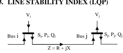
Fig. 1: Single line concept of power transmission

Voltage stability can be assessed in a system by calculating the line based voltage stability index. AMohamed et al[15] derived four line stability factors based on a power transmission concept in a single line. Out of these, the line stability index (LQP) is used in this paper. The value of line index shows the voltage stability of the system. The value close to unity indicates that the respective line is close to its stability limit and value much close to zero indicates light load in the line. The formulation begins with the power equation in a power system. Figure 1 illustrates a single line of a power transmission concept.

The power equation can be derived as;

𝑋

𝑉_𝑖2𝑄𝑖2− 𝑄𝑖+ _𝑉𝑋

𝑖2𝑃𝑖

2_{+ 𝑄}

𝑗 (1)

The line stability factor isobtained by setting the discriminant

of the reactive power roots at bus 1to be greater than or equal to zero thus defining the line stability factor, LQP as,

𝐿𝑄𝑃 = 4 𝑋 𝑉𝑖2

𝑋 𝑉𝑖2

𝑃𝑖2+ 𝑄𝑗 (2)

4.

PROBLEM FORMULATION

4.1

Static model of SVC

Fig. 2: Variable susceptance model of SVC

A variable susceptance BSVC represents the fundamental frequency equivalent susceptance of all shunt modules making up the SVC. This model is an improved version of SVC models. The circuit shown in figure 2 is used to derive the SVC's nonlinear power equations and the linearised equations required by Newton's load flow method. In general, the transfer admittance equation for the variable shunt compensator is

𝐼𝑆𝑉𝐶= 𝑗𝐵𝑆𝑉𝐶𝑉𝑗 (3)

And the reactive power is

𝑄𝑆𝑉𝐶 = −𝑉𝑗2𝐵𝑆𝑉𝐶 (4)

In SVC susceptance model the total susceptance BSVCis taken

to be the state variable, therefore the linearisedequation of the SVC is given by

∆𝑃𝑗 ∆𝑄𝑗 =

0 0 0 𝜃𝑗

∆𝜃𝑗

∆𝐵𝑠𝑣𝑐/𝐵𝑠𝑣𝑐 (5)

At the end of iteration i the variable shunt susceptance BSVCis

updated according to

𝐵_𝑆𝑉𝐶(𝑖) = 𝐵𝑠𝑣𝑐(𝑖−1)+ ∆BSVC/BSVC (𝑖)𝐵𝑆𝑉𝐶 (𝑖−1)

(6)

This changing susceptance value represents the total SVC susceptance which is necessary to maintain the nodal voltage magnitude at the specified value (1.0 p.u. in this paper).

4.2

Static model of TCSC

TCSC is a series compensation component which consists of a series capacitor bank shunted by thyristor controlled reactor. The basic idea behind power flow control with the TCSC is to decrease or increase the overall lines effective series transmission impedance, by adding a capacitive or inductive reactancecorrespondingly. TheTCSCis modeled as variable reactance shown in figure

3.

Xij = −0.8Xline ≤ XTCSC ≤ 0.2Xline 7

QSVC

Xline Vj

Vi

BSVC

Si, Pi, Qi Bus

j

i

Z = R + jX

Vi Vj

where, Xlineis the transmission line reactance, and XTCSC is the TCSC reactance.

Fig. 3: Model of TCSC

The level of the applied compensation of the TCSC usually varies between 20% inductive and 80% capacitive.

4.3

Objective function

The objective function of this work is to find the optimal rating and location of TCSC and SVC which minimizes the real power loss and maximizes the voltage stability limit, voltage deviation and line stability index. Hence, the objective function can be expressed as

𝐹 = 𝑀𝑖𝑛𝑖𝑚𝑖𝑧𝑒 𝑓1+ 𝜆1𝑓2+ 𝜆2𝑓3 (8)

The term f1 represents real power loss as 𝑓1= 𝐺𝑘[

𝑁𝐿

k=1

𝑉𝑖2+ 𝑉𝑗2− 2𝑉𝑖𝑉𝑗𝑐𝑜𝑠⁡(𝛿𝑖− 𝛿𝑗)] (9)

The term f2 represents total voltage deviation (VD) of all load

buses as

𝑓2= 𝑉𝐷 = (𝑉𝑖− 𝑉𝑟𝑒𝑓)2 𝑁𝑃𝑄

𝑘=1

(10)

The term f3 represents line stability index (LQP) as 𝑓3= 𝐿𝑄𝑃 = 𝐿𝑄𝑃𝑗

𝑁𝐿

𝑗 =1

(11)

where λ1 and is λ2 are weighing factor for voltage deviation

and LQP index and are set to 10.

The minimization problem is subject to the following equality and inequality constraints

(i) Load Flow Constraints:

𝑃𝐺𝑖− 𝑃𝐷𝑖− 𝑉𝑖𝑉𝑖𝑗𝑌𝑖𝑗cos 𝛿𝑖𝑗+ 𝛾𝑗 − 𝛾𝑖 = 0 𝑁𝐵

𝑗 =1

(12)

𝑄𝐺𝑖− 𝑄𝐷𝑖− 𝑉𝑖𝑉𝑖𝑗𝑌𝑖𝑗sin 𝛿𝑖𝑗+ 𝛾𝑗 − 𝛾𝑖 = 0 𝑁𝐵

𝑗 =1

(13)

(ii) Reactive Power Generation Limit of SVCs:

𝑄𝑐𝑖𝑚𝑖𝑛 ≤ 𝑄𝑐𝑖≤ 𝑄𝑐𝑖𝑚𝑎𝑥; 𝑖 ∈ 𝑁𝑆𝑉𝐶 (14)

(iii) Voltage Constraints:

𝑉𝑖𝑚𝑖𝑛 ≤ 𝑉𝑖≤ 𝑉𝑖𝑚𝑎𝑥; 𝑖 ∈ 𝑁𝐵 (15)

(iv) Transmission line flow limit:

𝑆𝑖≤ 𝑆𝑖𝑚𝑎𝑥; 𝑖 ∈ 𝑁𝑙 (16)

4.4

Shuffled Frog Leaping Algorithm – An

Over view

The SFLA is a meta-heuristic optimization method which is based on observing, imitating, and modeling the behavior of a group of frogs when searching for the location that has the maximum amount of available food. SFLA, originally

developed by Eusuff and Lansey in 2003[16], can be used to solve many complex optimization problems, which are nonlinear, non differentiable, and multi-modal. The SFLA combines the benefits of the both the genetic-based memetic algorithm and the social behavior-based PSO algorithm

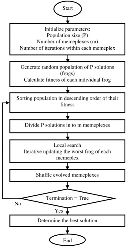
Fig. 4: Flow chart of Shuffled Frog Leaping Algorithm

In SFLA, there is a population of possible solutions defined by a set of virtual frogs partitioned into different groups which are described as memeplexes, each performing a local search. Within each memeplex, the individual frogs hold ideas, which can be infected by the ideas of other frogs. After a defined number of memetic evolution steps, ideas are passed between memeplexes in a shuffling process. The local search and the shuffling process continue until the defined convergence criteria are satisfied.The flow chart of shuffled frog leaping algorithm is depicted in fig 4.

In the first step of this algorithm, an initial population of P frogs is randomly generated within the feasible search space. The position of the i th frog is represented as Xi = (Xi1, Xi2….XiD), where D is the number of variables. Then, the frogs are sorted in descending order according to their fitness.

Afterwards, the entire population is partitioned into m subsets referred to as memeplexes each containing n frogs (i.e., P = m x n). The strategy of the partitioning is as follows:

No

Yes Start

Initialize parameters: Population size (P) Number of memeplexes (m) Number of iterations within each memeplex

Generate random population of P solutions (frogs)

Calculate fitness of each individual frog

Sorting population in descending order of their fitness

Divide P solutions in to m memeplexes

Local search

Iterative updating the worst frog of each memeplex

Shuffle evolved memeplexes

Termination = True

Determine the best solution

End -jBsh

Bus j

-jBsh

Zij = Rij + Xij

-jXTCSC

The first frog goes to the first memeplex, the second frog goes to the second memeplex, the m th frog goes to the m th memeplex, the (m + 1) th frog goes back to the first memeplex, and so forth.

In each memeplex, the positions of frogs with the best and worst fitnesses are identified as Xb and Xw, respectively. Also the position of a frog with the global best fitness is identified as Xg.

Then, within each memeplex, a process similar to the PSO algorithm is applied to improve only the frog with the worst fitness (not all frogs)in each cycle. Therefore, the position of the frog with the worst fitness leaps toward the position of the best frog, as follows:

𝐷𝑖= 𝑟𝑎𝑛𝑑 × 𝑋𝑏− 𝑋𝑤 (17)

𝑋𝑤𝑛𝑒𝑤 = 𝑋𝑤𝑜𝑙𝑑+ 𝐷𝑖 𝐷𝑖 𝑚𝑖𝑛 < 𝐷𝑖< 𝐷𝑖 𝑚𝑎𝑥 (18)

where Dimax and Dimin are the maximum and minimum step sizes allowed for a frog‟s position, respectively.

If this process produces a better solution, it will replace the worst frog. Otherwise, the calculations in (17) and (18) are repeated but are replaced but Xb is replaced by Xg. If there is no improvement in this case, a new solution will be randomly generated within the feasible space to replace it. The calculations will continue for a specific number of iterations. Therefore, SFLA simultaneously performs an independent local search in each memeplex using a process similar to the PSO algorithm. After a predefined number of memetic evolutionary steps within each memeplex, the solutions of evolved memeplexes are replaced into new population shuffling process.

The shuffling process promotes a global information exchange among the frogs. Then, the population is sorted in order of decreasing performance value and updates the populationbest frog‟s position, repartition the froggroupinto memeplexes, and progress the evolution within each memeplex until the conversion criteria are satisfied. Usually, the convergence criteria can be defined as follows:

The relative changes in the fitness of the global frog within a number of consecutive shuffling iterations are less than a pre-specified tolerance.

The maximum predefined number of shuffling iteration has been obtained. The optimal parameter values of shuffled frog leaping algorithm shown in table 1.

4.5

Implementation of Shuffled Frog

Leaping Algorithm

Step 1: Select m the number of memeplexes and n the

number of frogs in each memeplex. Total frogs P = m x n. Generate required population (Xi), i=1 to P, by random generation. Evaluate the fitness f (Xi) of each frog and arrange them in ascending order.

Step2: According to the fitness value, arrange the frogs in to memeplexes (The first frog goes to the first memeplex, the second frog goes to the second memeplex, the m th frog goes to the m th memeplex, the (m + 1) th frog goes back to the first memeplex, and so forth.). Find the position of frogs with the best, worst fitnesses identified as Xb and

Xw respectively and the global best Xg for all m-memeplexes.

Step 3: Improving worst frog position: The local exploration is implemented in each memeplex, i.e., the worst performance frog (Xw) in the memeplex is updated according to the following modification rule: Di = rand x (Xb - Xw) , i=1 to m. Accept Di if it is within Dmin and Dmax, i.e.; Dmin < Dm< Dmax, otherwise set to minimum or maximum limits of Di. „rand‟ is the random number generated between 0 and 1. The new position of the frog is updated as

Xw new

= Xw old

+ Di ; (Dmin < Dm< Dmax). Then recalculate fit of this frog.

Step 4: If the fitness of Xw new

is more than the fitness of Xw

old

then accept the Xw new

. Else generate new Di value with respect to global Xg :

Di = Rand x (Xb - Xw). Accept Di if it is Dmin and

Dmax, otherwise set to minimum or maximum limits of Di. The new position is computed by

Xw new

= Xw old

+ Di. Again compute fitness of this

frog.

If the fitness of Xw new

is more than the fitness of Xw

old

then accept the Xw new

. Else randomly generate the new frog in place of Xw within the acceptable frog limits.

Step 5: Repeat step 3 and 4 for all memeplexes. This completes one iteration. Now shuffle the frogs as per step 2.

Step 6: Repeat algorithm until the solution criterion is met or maximum number of iterations are completed. The solution criterion is [|Xwnew | - | Xwold |] < Є, where Є is the convergence tolerance. Stop.

Table 1. Optimal values of SFLA parameters

Parameters Optimal value

Number of frogs 50

Number of memeplexes 5

Number of frogs per memeplexes 10

5.

RESULTS AND DISCUSSIONS

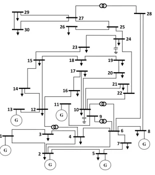
Figure 5: One line diagram of IEEE 30 Bus Test System

The proposed work is coded in MATLAB 7.6 platform using 2.8 GHz Intel Core 2 Duo processor based PC. The method is tested in the IEEE 30 bus test system shown in figure 5.The line data and bus data are taken from the standard power system test case archive. The system has 6 generator buses, 24 load buses and 41 transmission lines. System data and results are based on 100 MVA and bus1 is the reference bus. In order to verify the presented models and illustrate the impacts of TCSC and SVC study, two different stressed conditions are considered as mentioned below.

Case 1: The system with 50 % increased load in all the load buses is considered as a critical condition due to increased load. Loading of the system beyond this level, results in poor voltage profile in the load buses and unacceptable real power loss occurs.

Case 2: Contingency analysis carried out on the IEEE 30 bus system shows that line number 5 connected between buses 2 and 5 is the most critical line. The systemwith outage of line number 5 is taken as stressed conditions due to line outage.

In case 1, the Newton – Raphson program is repeated with presence and absence of TCSC and SVC devices. The LQP values of all lines under normal and critical loading conditions are depicted in figures 6 and 7 respectively.

Figure 6: LQP index values under normal loading

In case 2, the line outage is ranked according to the severity and the severity is taken on the basis of the line stability index values (LQP) and such values are arranged in descending order. The maximum value of index indicates most critical line outage. Line outage contingencyscreening and ranking is carried out on the test system and the results are shown in table 2. It isclear from theresultsthat outage of line number 5 is the most critical line outage and this

0 0.2 0.4 0.6

1 4 7 10 13 16 19 22 25 28 31 34 37 40

LQ

P

In

d

ex

V

a

lu

es

Line Number

Without TCSC and SVC With TCSC and SVC 1

30

29 ₂₈

27

20

21

22 23

24

26 25

19 18

17

16 15

14

13 12 11 10

9

8

7 6

5 4

3

2

G

G G

G G

condition is considered for voltage stability improvement. Outage of other lines has no much impact on the system and therefore they are not given importance.

Figure 7: LQP index values under critical loading

The details of voltage profiles in all cases are shown in table 3 and the corresponding values of LQP index are depicted in figure 8. It is clear from the table that the voltage profile is improved considerably. The sum of LQP values in all cases is also depicted in figure 9.

Table 2. Contingency Ranking

Rank Line

Number LQP index Values

1 5 0.9495

2 9 0.6050

3 2 0.4993

4 4 0.4968

5 7 0.4693

6 6 0.3965

7 10 0.3960

8 15 0.3943

9 3 0.3940

10 11 0.3917

Table 3. Voltage Profile Values of all cases

Bus No.

Normal Loading Critical Loading

Single Line Outage Contingency Condition Without TCSC and SVC With TCSC and SVC Without TCSC and SVC With TCSC and SVC Without TCSC and SVC With TCSC and SVC

1 1.0600 1.0600 1.0600 1.0600 1.0600 1.0600

2 1.0400 1.0430 1.0030 1.0030 1.0430 1.0430

3 1.0217 1.0225 0.9745 0.9764 1.0069 1.0105

4 1.0129 1.0139 0.9581 0.9605 0.9958 1.0003

5 1.0100 1.0100 0.9600 0.9600 0.9600 0.9600

6 1.0121 1.0130 0.9553 0.9574 0.9909 0.9977

7 1.0035 1.0040 0.9438 0.9451 0.9661 0.9753

8 1.0100 1.0100 0.9600 0.9600 0.9900 1.0000

9 1.0507 1.0548 0.9923 1.0020 1.0388 1.0425

10 1.0438 1.0517 0.9722 0.9856 1.0366 1.0345

11 1.0820 1.0820 1.0520 1.0620 1.0820 1.0820

12 1.0576 1.0612 1.0004 1.0101 1.0495 1.0520

13 1.0710 1.0710 1.0410 1.0510 1.0710 1.0710

14 1.0429 1.0480 0.9754 0.9859 1.0339 1.0367

15 1.0385 1.0449 0.9670 0.9786 1.0288 1.0313

16 1.0445 1.0500 0.9769 0.9882 1.0341 1.0372

17 1.0387 1.0459 0.9650 0.9778 1.0262 1.0299

18 1.0282 1.0352 0.9489 0.9614 1.0167 1.0201

19 1.0252 1.0326 0.9434 0.9563 1.0131 1.0167

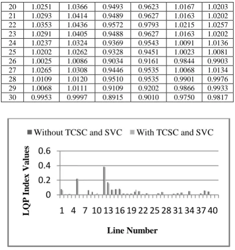
20 1.0251 1.0366 0.9493 0.9623 1.0167 1.0203

21 1.0293 1.0414 0.9489 0.9627 1.0163 1.0202

22 1.0353 1.0436 0.9572 0.9793 1.0215 1.0257

23 1.0291 1.0405 0.9488 0.9627 1.0163 1.0202

24 1.0237 1.0324 0.9369 0.9543 1.0091 1.0136

25 1.0202 1.0262 0.9328 0.9451 1.0023 1.0081

26 1.0025 1.0086 0.9034 0.9161 0.9844 0.9903

27 1.0265 1.0308 0.9446 0.9535 1.0068 1.0134

28 1.0109 1.0120 0.9510 0.9535 0.9901 0.9976

29 1.0068 1.0111 0.9109 0.9202 0.9866 0.9933

30 0.9953 0.9997 0.8915 0.9010 0.9750 0.9817

Figure 8: LQP index values under single line outage contingency condition

Figure 9: Sum of LQP index values in all cases

For installation of TCSC, the candidate positions are the lines without tap changing transformer. The lines 11, 12, 15 and 36 are with tap changing transformer and not considered for positioning of TCSC. Locating TCSC on different branches is tried one by one based on the proposed algorithm. SVC can be connected only to load buses. Buses 1, 2, 5,8,11 and 13 are generator buses and therefore not considered as possible locations for SVC. When the global best position for an TCSC is a line with tap changing transformer or global best position of an SVC is a generator bus then the position is relocated to a geographically closer line without transformer or load bus. The most suitable location for TCSC to control power flow is found to be line number 21 for normal loading and line number 22 and 7 for critical loading and line outage contingency conditions respectively. Similarly SVC to improve voltage profile are found to be bus number 2 for normal loading and bus number 20 for both critical loading and line outage contingency conditions.

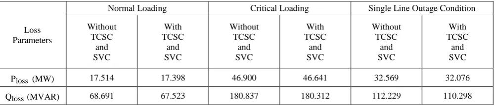
In loss minimization point of view through insertion of TCSC and SVC, the real power loss under normal loading is decreased by 0.116 MW which is 0.67% of total real power loss. Similarly under critical loading and line outage contingency conditions the real power loss decreased by 0.259

0 0.2 0.4 0.6

1 4 7 10 13 16 19 22 25 28 31 34 37 40

LQ P In d ex v a lu es Line Number

Without TCSC and SVC With TCSC and SVC

0 0.2 0.4 0.6

1 4 7 10 13 16 19 22 25 28 31 34 37 40

LQ P In d ex V a lu es Line Number

Without TCSC and SVC With TCSC and SVC

1.4722 2.5236 1.6931 1.4039 2.4693 1.6229 0 1 2 3

Normal Critical Contingency

S u m o f LQ P In d ex V a lu es

Table 4. Real and Reactive power Loss Values for all cases

Loss Parameters

Normal Loading Critical Loading Single Line Outage Condition

Without TCSC

and SVC

With TCSC

and SVC

Without TCSC

and SVC

With TCSC

and SVC

Without TCSC

and SVC

With TCSC

and SVC

Ploss (MW) 17.514 17.398 46.900 46.641 32.569 32.076

Q_loss(MVAR) 68.691 67.523 180.837 180.312 112.229 110.298

Table 5. Best Location of TCSC and SVC

Cases

TCSC SVC

Location Degrees

of Compensation Location Size (MVAR)

Normal loading Between buses 16 and 17 (Line 21) -0.0873 Bus No. 2 9.2532

Critical loading Between buses 15 and 18 (Line 22) -0.2811 Bus No. 20 8.2923

Single line outage contingency Between buses 4 and 6 (Line 7) -0.6438 Bus No. 20 9.8308

MW and 0.493 MW respectively. The percentages of reduction under these cases are 0.55% and 1.51 % respectively. The real and reactive power losses under all cases are shown in table 4. The reduction in real power loss and increase in voltage magnitudes after the insertion of TCSC and SVC proves that FACTS devices are highly efficient in relieving a power network from stressed condition and improving voltage stability limit.

The best location and size (Degrees of compensation) of TCSC under all conditions are shown in table 5. The location of TCSC is quiet different in all cases. But the best location of SVC is same under critical loading and contingency conditions and not same under normal loading condition. The size of SVC is not so large and lies between 8.2923 MVAR to 9.8308 MVAR which helps to minimize the cost of VAR devices. The size of SVC is least under critical loading condition.

6.

CONCLUSIONS

In this paper, optimal location of TCSC and SVC for voltage stability limit improvement and loss minimization are demonstrated. The voltage stability limit improvement and real power loss minimization are done under critical loading and line outage contingency conditions. The LQP index is

used for voltage stability assessment. The reactance model of TCSC is considered to improve the voltage stability limit by controlling power flows and maintaining voltage profile. The performance of TCSC and SVC combination in optimal power flow control for voltage stability limit improvement is proved in the results by comparing the system real power loss and voltage profile with and without the devices. It is clear from the numerical results that voltage stability limit improvement is highly encouraging. The voltage stability limit improvement is by the combined action of power flow control of TCSC and reactive power compensation by SVC.

7.

REFERENCES

[1] Voltage stability of power systems: concepts, analytical tools, and industry experience, IEEE Special Publication 90TH0358-2-PWR, 1990.

[2] T. V. Cutsem, “Voltage instability: Phenomena, countermeasures, and analysis methods,” Proceedings of the IEEE, vol. 88, pp. 208–227, February 2000.

[3] C. W. Taylor, Power System Voltage Stability. New York: McGraw-Hill, 1994P.

[4] P.Kundur, Power System stability and control, McGraw-Hill, 1994.

[5] L.H. Fink, ed., Proceedings: Bulk power system voltage phenomena III, voltage stability, security & control, ECC/NSF workshop, Davos, Switzerland, August 1994.

[6] I. Dobson, H.-D. Chiang, “Towards a theory of voltage collapse in electric power systems”, Systems and Control Letters, vol. 13, 1989, pp. 253-262.

[7] CIGRE Task Force38-0210,”Modelling of Voltage Collapse Including Dynamic Phenomena, CIGRE Brochure, No 75, 1993.

[8] Technical Analysis of the August 14, 2003, Blackout: What Happened, Why, and What Did We Learn? A report by the North American Electrical Reliability Council Steering Group, July 13, 2004.

[9] N G. Hingorani, L. Gyugyi, Understanding FACTS: Concepts and Technology of Flexible ACTransmission Systems, IEEE Press, New- York, 2000.

[11]Musunuri, S, Dehnavi, G, “Comparison of STATCOM, SVC, TCSC, and SSSC Performance in Steady State Voltage Stability Improvement” North American Power Symposium (NAPS), 2010.

[12]C.A.Canizares, Z.Faur, “Analysis of SVC and TCSC Controllers in Voltage Collapse”, IEEETransactions on power systems, Vol.14, No.1, Feb 1999, pp.158-165. [13]MaysamJafari,Saeed Afsharnia,”Voltage Stability

Enhancement in Contingency Conditions using Shunt FACTS Devices”,EUROCON - The international conference on computer as a tool,Warsaw,Sep 9-12,IEEE,2007.

[14]Claudia Reis, Antonio Andrade and F.P.Maciel, “Line Stability Indices for Voltage Collapse Prediction”, IEEE Power Engineering conference, Lisbon, Portugal, March. 2009.

[15]A.Mohmed, G.B.Jasmon and S.Yusoff, “A static voltage collapse indicator using line stability factors”, Journal of industrial technology, Vol.7, No.1, pp.73 – 85, 1989. [16]M. M. Eusuff, K. E. Lansey, and F. Pasha, “Shuffled

frog-leaping algorithm: A memetic meta-heuristic for discrete optimization,” Engg. Optimization. Vol. 38, no. 2, pp. 129–154, 2006.

[17]Eusuff, M. M., and Lansey, K. E., “Optimization of Water Distribution Network Design Using the Shuffled Frog Leaping Algorithm”, Journal of Water Resources Planning and Management, 2003, Vol 129, No.3, pp. 210-225

[18]N.D.Reppen, R.R.Austria, J.A.Uhrin, M.C.Patel, A.Galatic,”Performance of methods for ranking a evaluation of voltage collapse contingencies applied to a large-scale network”, Athens Power Tech, Athens, Greece, pp.337-343, Sept.1993.

[19]G.C. Ejebe, G.D. Irisarri, S. Mokhtari, O. Obadina, P. Ristanovic,J. Tong, Methods for contingency screening and ranking for voltage stability analysis of power systems, IEEE Transactions on Power Systems, Vol.11, no.1, Feb.1996, pp.350-356.

[20]E.Vaahedi, et al “Voltage Stability Contingency Screening and Ranking”, IEEE Transactions on power systems, Vol.14, No.1, February 1999.

[21]S.Sakthivel, D.Mary, “Voltage stability limit improvement incorporating SSSC and SVC under line outage contingency condition by loss minimization”, European journal of scientific research, Vol.59, No.1, 2011, pp. 44 – 54.

8.

AUTHOR’S PROFILE

L. Jebaraj received the Degree in Electrical and Electronics Engineering from The Institution of Engineers (India), Kolkata and Masters Degree (Distn.) in Power Systems Engineering from Annamalai University, Chidambaram, India in 1999 and 2007 respectively. He is doing the Ph.D., Degree in Electrical Engineering faculty from Anna University of Technology, Tiruchirappalli, India. He is working as an Assistant Professor of Electrical and Electronics Engineering at V.R.S. College of Engineering and Technology, Villupuram, Tamil Nadu, India. His research areas of interest are Power System Optimization Techniques, Power system control, FACTS and voltage stability studies.

C.Christober Asir Rajan received the B.E. Degree (Distn.) in Electrical and Electronics Engineering and Masters Degree (Distn.) in Power Systems Engineering from Kamaraj University, Madurai, India in 1991 and 1996 respectively. He received his Ph.D Degree in Electrical Engineering faculty from Anna University, Chennai, India in 2004. He is currently working as an Associate Professor in Electrical and Electronics Engineering Department at Pondicherry Engineering College, Puducherry, India. His area of interest is power system optimization, operation, planning and control. He is a member of ISTE and the institution of engineers (India).