Downside Risk for European Equity Markets

Munich Personal RePEc Archive

Downside Risk for European Equity

Markets

Cotter, John

2004

Online at

https://mpra.ub.uni-muenchen.de/3537/

Downside Risk for European Equity Markets

JOHN COTTER University College Dublin

Abstract

This paper applies extreme value theory to measure downside risk for European equity markets. Two related measures, value at risk and the excess loss probability estimator provide a coherent approach to optimally protect investor wealth opportunities for low quantile and probability combinations. The fat-tailed characteristic of equity index returns is captured by explicitly modelling tail returns only. The paper finds the DAX100 is the most volatile index, and this generally becomes more pronounced as one moves to lower quantile and probability estimates.

Keywords: risk estimation, extreme value theory, fat-tailed equity returns.

Address for Correspondence:

Dr. John Cotter,

Centre for Financial Markets,

Department of Banking and Finance, Graduate School of Business,

University College Dublin, Blackrock,

Co. Dublin, Ireland.

Downside Risk for European Equity Markets

I INTRODUCTION

Recently downside risk has become a highly debated topic, recognising the need for

appropriate risk management practices given that systematic risk cannot be

eliminated.1 Amongst the methods applied are mean variance analysis (portfolio

theory) and Value at Risk (VaR). The use of these approaches aims to control downside risk so as to maximise investor wealth opportunities. Portfolio theory

examines a risk return trade-off for different combinations of assets in order to

control risk for given return levels. Similarly, VaR focuses on a maximum level of

loss that investors would be willing to incur given the returns distribution. This

quantile measure gives investors specific information on the degree of downside

risk at a number of probabilities and horizons (for example, a single VaR statement

might indicate that an investment’s losses should not exceed 5% for a 10 day

holding period and at the 95% confidence level).2 In a risk management context,

the uniform aim of both approaches is to control the possible losses that the investor

may encounter.

This paper uses a semi-parametric methodology, extreme value theory, to quantify

tail behaviour for European equity indexes in a VaR framework. Alternatively,

time series analysis has focused on the full distribution of returns testing the

random walk and mean reversion hypotheses (Gallagher, 1999). Relating to VaR

measurement, a number of studies have examined equity returns series to determine

and Taylor). Diverging support is offered regarding a number of separate

hypotheses including ARCH and stable paretian related distributions. Extreme

value theory nests both hypotheses thereby providing a unique approach to

distinguish between the alternative distributions. Nevertheless, all the studies agree

that the financial data analysed exhibits fat tails relative to the normal distribution.

This characteristic can lead to problems in VaR computations if one assumes a

distribution that does not exactly fit the data under analysis. In particular, assuming

gaussian properties for equity index returns leads to an underestimation of the tail index, and consequentially their counterparts, the VaR measures. Making use of

extreme value theory that specifically models tail behaviour only, and allowing for

the case of fat tails gives greater precision to the lower quantile VaR estimates

(Diebold et al., 1998).

Furthermore, a series' of papers have focused on various issues regarding VaR

computations (Danielsson and DeVries, 1997a, 1997b, 2000; Kearns and Pagan,

1997; Duffie and Pan, 1997; Venkataraman, 1997; and Loretan, and Phillips, 1994).

The findings offer further support in the use of extreme value theory as the most

appropriate method in calculating VaR estimates; the Hill (1975) statistic as being

the optimal tail estimate; and that the properties of extreme returns are unlike the full series of returns. Moreover, VaR theoretically suffers from an inability to

measure risk beyond the chosen quantile (Artzner et al., 1999). Thus, to provide a

coherent description of downside risk there is a need for a measure that goes

beyond the VaR. This paper outlines and measures a new statistic, the excess loss

probability estimator for examining this issue. This estimator measures the

The outline of the paper is set out as follows. Section II deals with theoretical and

methodological issues. Initially a description of related VaR measures are given.

This is followed by a debate on the relative merits of extreme value theory. Section

II is concluded with a presentation of the main theoretical and methodological

findings of extreme value theory. Then a description of the data is given in the

third section, showing preliminary statistics for the indexes analysed, as well as a

snapshot of the extreme returns. Results are presented and discussed in section IV. Finally, conclusions are detailed in section V.

II THEORITICAL AND METHODOLOGICAL ISSUES

Value at Risk (VaR)

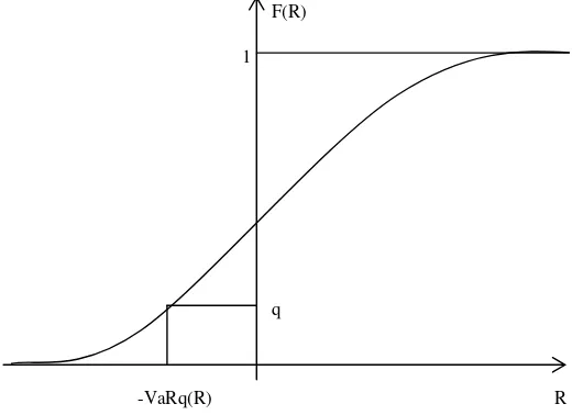
Value at Risk (VaR) is a statistical measure of (downside) risk that estimates the

maximum loss that may be experienced by a portfolio (index) over a given period

with a given confidence level. Taking a random variable R, representing the set of

index returns, with distribution function F detailing all positive and negative returns

over a prespecificied time period, its risk can be defined by a VaR estimate. The

VaRq is the qth quantile of the distribution of negative returns

VaRq = -F-1(q) (1) where F-1(q) is the quantile function and is the inverse function of F.

Graphically, the VaRq is represented in figure 1 with the quantile cut-off point VaR

(R) measuring the maximum loss for that given quantile.

However the VaR measure cannot be considered as a panacea for risk management

estimation. While (1) gives a measure for the amount of possible downside risk

exposure upto the extreme negative return, r, it has been criticised for not

describing the losses in excess of the VaRq that an investor can incur (Artzner et

al., 1999). We would expect a priori that a risk averse investor is similarly

ill-disposed (or even more so) to losses in excess of the VaR as they are to the measure

itself. For instance, considering figure 1 the VaR estimate does not tell us anything

about returns further out in the tail, those values that can be considered as the Excess Loss (ELp) of the VaR. Thus to provide a coherent picture of downside risk

we should also examine the probability of having excess losses greater that a VaR

threshold by focusing on the probability mass to the left of VaR in figure 1.

Formally this is given as

ELp = P[R | R > VaRq] (2)

for extreme (negative) returns.

The most controversial element of the Riskmetrics system is the assumption that the

unconditional distribution of financial returns follows a normal distribution.

However one of the main stylized facts for financial time series is the rejection of

normality (see findings later for our equity indexes). Moreover, the empirical features all to some degree indicate volatility clustering, and there is evidence that

this characteristic of financial time series impinges on the efficiency of the tail

estimates (Duffie and Pan, 1997). In particular, parametric approaches including

portfolio theory (variance-covariance analysis) underestimate extreme returns,

regardless of whether they are located in the upper or lower tail of the distribution.

estimated are greater for the true data generating processes, than that of their

gaussian counterpart. This conclusion can be clearly seen for any quantile by

focusing on the downside tail returns given in figure 2. Here, the empirical

distribution of equity index returns (shaded curve), following a fat tailed process, is

plotted against the normal distribution (solid curve), following a relatively thin

tailed process. At all times, the normal distribution underestimates the downside

tail behaviour vis-à-vis the fat tailed process.

INSERT FIGURE 2 HERE

Furthermore, a case study will emphasise the magnitude of the underestimation

issue. For instance a clear example of the tails from a normal distribution

underestimating downside risk is the case of the stock market crash, 19 October

1987. Here, most international equity markets showed actual losses in excess of

10%. However, under gaussian assumptions, such an occurrence would only occur

once every 5900 years (Venkataraman, 1997). Obviously empirical evidence is

contrary to this forecast showing greater losses being recorded in a shorter time

frame, for example, the occurrence of the crash of1929. A similar conclusion can

be made for any large negative loss in any asset market. The most common

measure actually applied in relation to tail densities is the centred kurtosis statistic, the fourth moment of a distribution. For the normal distribution, this estimate takes

on a value of 0, whereas in the presence of platykurtosis, thin tails, the value is less

than 0. Leptokurtosis is consistent with relatively fat tails relative to the gaussian

Debate on Extreme Value Theory:

As we have seen with gaussian estimation of tail values the primary empirical

consideration in using the VaR approach is to apply the most efficient estimation

technique. This paper picks the extreme value theory (see Leadbetter et al., 1983,

for a comprehensive discussion) at the expense of the more traditional methods of

the variance-covariance approach, historical simulation and Monte Carlo

simulation. Its approach lies in calculating a lower tail percentile from the

distribution of returns for some prespecified time period. This is equivalent to focusing on the large losses of an investment, that is, the maximum downside of

risk.

There has been considerable debate of the relative strengths and weaknesses of

using extreme value theory in examining tail behaviour (Diebold et al., 1998).

Both theoretical and practical issues have been the focus of discussion. This paper

briefly presents a synopsis of these and examines those of relevance to the

empirical application at hand. To begin, turning to the strengths, an application of

extreme value theory does not suffer from model risk in comparison to the variance

covariance approach (standard portfolio theory) and Monte Carlo methods. These

alternative approaches examine probabilities for the full distribution of returns, whereas the actual focus of attention, the tail values are explicitly modelled

separately by extreme value theory. Thus for instance, we always end up with

underestimation of tail behaviour by applying the variance covariance approach,

and result in inappropriate tail estimates with Monte Carlo simulation of alternative

full distributions such as the student-t process (see Cotter, 2001; for an illustration).

analysis is required. Alternatively simulation has been used to examine different

(worse case) scenarios. These however are subjectively defined and unlike the

application of extreme value theory, they do not define an objective likelihood

function.

A key addition that extreme value theory makes is that it removes the need for

making assumptions as to the exact distributional form of the data under analysis.

It separates out three types of distribution of which financial returns belong to the fat tailed classification. This is because under extreme value theory all fat tailed

distributions have the same limit law and thus the correct distributional form is not

a primary concern. Briefly, this limit law induces an identical feature in fat tailed

realisations as they exhibit a regular variation property. Feller (1971) found that

this regular variation at infinity property is the sufficient and necessary property for

fat tailed distributions to hold. It implies that not all moments of the fat tailed

distribution are bounded unlike other types of distributions such as normality.

Furthermore extreme value estimates can easily be extended from a certain observation frequency, for example daily to weekly estimates (see Jansen et al.,

2000; for an illustration). This extension is similar to the scaling law of normality where lower frequency estimates follow a square root of time rule. Both

approaches do not require any further estimation and there is no need for additional

observations measured at different frequencies. Thus for instance, daily extreme

value estimates can easily be scaled up for weekly estimates without estimating

procedure that is applied in this study, which can be impaired for smaller sample

sizes, that is by examining data sets at lower frequencies.3

Finally, our semi-parametric tail estimation procedure can be extended for

out-of-sample periods (see empirical illustration later). This allows us to give very low

probability tail estimates and thus dominate the historical simulation approach that

is restricted to probabilities (1/n) within the sample size, n. Thus the downside risk

measures presented go beyond the sample size estimated, for example using 5 years of data to obtain downside risk forecasts for a 10 year period. Thus, these

out-of-sample forecasts remove the data size restrictions that impair many empirical

studies.

Notwithstanding the attractive features of extreme value theory, there are a number

of potential weaknesses of the approach. First, the statistical theory on the

properties of the finite-sample Hill index (our downside tail estimator) is as yet not

fully developed although it is consistent and asymptotically normal for infinite

samples. Furthermore, the Hill index is used indirectly in risk management

estimation as it is extreme probability and quantile estimates that are presented.

These estimates are non-linear functions of the Hill index, and as a consequence of any poor statistical properties of this measure, would themselves suffer suboptimal

statistical features. Second, much of extreme value theory has been presented for

an identical and independently distributed variable, in contradiction to the volatility

clustering inherent in financial returns. However, the theory has been extended to

deal with a stationary case (see Leadbetter et al., 1983). This property is accepted

generally assumed that financial returns are in the maximum domain of attraction of

a Fréchet distribution implying that the tail follows a power law. However,

financial variables such as those relating to credit risk estimation do not have fat

tailed features. Thus it is necessary to first ensure that the stock index returns

analysed are fat tailed by examining their centred kurtosis statistic and the value of

the Hill tail index.

Extreme Value Estimation:

The key addition that extreme value theory makes to downside risk analysis is that

it removes the need for making assumptions as to the exact distributional form of

the data under analysis. The asset returns series may follow any fat tailed

distribution such as a stable paretian or mixtures of normals, but at the limit they all

converge to the same underlying distribution. As the same limit law applies, the

correct distributional form of the asset returns is not a primary concern. For the

fat-tailed case, returns are assumed to belong to the maximum domain of attraction of

the Fréchet distribution. This result follows a similar role as the central limit

theorem and normality but here asymptotically the returns converge to the fat tailed

distribution.4 To overcome the lack of an exact fit for the finite equity index returns this study uses a semi-parametric tail estimator, the moments based Hill estimator.

Formally, taking a sequence of strictly stationary returns {R1, R2,..., Rn}that may,

but not necessarily be identical and independently distributed (Leadbetter et al.,

returns, we can examine the minima (Mn) of a sequence of n random variables

rearranged in ascending order where

Mn = Min{ R1, R2,..., Rn} (3)

where Mn is an order statistic

and

P{Mn ≤ r} = P{R1 ≤ r, …, Rn≤ r} = F(r) -∞ < r < ∞ (4)

The random variables of interest in this analysis, the negative returns, are located at

the tail of the distribution, F(r). For example, the VaR measures the amount of

possible loss exposure upto the extreme return, r. Losses in excess of this extreme

return can be generated, and related measures of the probability of exceeding the

extreme return, r, are given by Excess Loss (ELp) estimators for a range of possible

losses.

As stated we model our fat tailed returns to be in the maximum domain of attraction

of the Fréchet distribution. In fact, extreme value theory examines three alternative types of tail behaviour. There is a type I process where variables are in the

maximum domain of attraction of a Gumbell distribution. Here the tail declines

exponentially and all the moments of the distribution are bounded. Examples of

this process include the commonly used normal and log normal distributions where

the fast tail decline results in thin tailed distributions. Furthermore, there is a type

III process where variables are in the maximum domain of attraction of a Weibull

distribution. Here there is no tail defined in the sense that there is no observed

values beyond a certain threshold at the end of a distribution, of which the uniform

In contrast, the fat tailed Fréchet distribution follows a type II process where the tail

has a power decline resulting in all moments not necessarily being defined:

Type II (Fréchet): F(-r) = = exp (r)-α (5)

where 1/α is the value of the tail index and is assumed positive.

The power decline of a type II process induces a relatively slow decay for

convergence at the limit vis-à-vis the relatively faster decline of the type I process

with the stable paretian and student-t processes representing specific cases. The tail

index, 1/α, can take on a number of interpretations if an underlying distribution is

assumed for the random variable (returns) being analysed. For instance, if the data

belongs to the family of stable paretian distributions, 1/α is a measure of the

characteristic exponent of the stable distribution, whereas, for the student-t

distribution, 1/α is a measure of the number of degrees of freedom. Equation (5)

indicates that for fat-tailed distributions, an estimate of the tail index, 1/ , is used to

develop risk measures such as VaR computations and their inferences.

All fat tailed distributions have a common characteristic by having a regular variation at infinity property:

Type II (Fréchet): lim F(-tr) = r-α (6) t →∞ F(-t)

for α > 0.

This is the sufficient and necessary condition for fat-tailed distributions to hold (Feller, 1971). Assuming that (5) holds, and the random variable under

consideration is fat tailed, then a first order approximation of its tail distribution is

given as:

P{R > r} ≅ ar(-α), a > 0, α > 0 (7)

A more detailed parametric form of the tail for all fat tailed type distributions can

be obtained by taking a second order expansion:

F(-r) = 1 - ar(-α) [1 + br-β+ 0(r-β)], β > 0, as r →∞ (8)

β and b are second order equivalents to α and a.

From (8), a related tail index estimator can be developed based on order statistics so

that the tail values are compared to some threshold value, m.

Kearns and Pagan (1997) find that the moments based Hill (1975) estimator dominates other approaches, and in particular, the Hill index does not suffer from

small sample bias and is relatively more efficient. The Hill estimator uses order

statistics as opposed to averages:

γˆ = 1/α = (1/m) [log R(n + 1 - i) - log R(n - m)] for i = 1....m (9)

where Ri are the lowest (negative) order statistics. The tail estimator is

asymptotically normal, (γ - γˆ )/(m)1/2 ≈ (0, γ2). The Hill estimator represents a

semi-parametric measure detailing tail behaviour only rather than examining the

full distribution of returns using the inferior fully parametric approaches. For the

VaR analysis, it is necessary to understand the maximum loss for a specified period, but also, it is advantageous to determine if there is stability in this measure. This

would allow us to extend the analysis from downside risk measures to upside risk

measures (dealing with short positions). Tail stability testing is based on a Loretan

and Phillips (1994) test statistic:

V(γ+ - γ-) = [γ+ - γ-]2/[γ+2/m+ + γ-2/m-]1/2 (10)

for γ+ (γ-) is the estimate of the right (left) tail, and the statistic asymptotically

Using (9) to determine the tail index, various VaR quantile estimates can be

generated using the following:

qt = R(m)(m/nt)γ (11)

This allows the development of VaR type statements. The quantiles measured by

(11) shows the maximum loss for different confidence levels. It can be used to

determine the extent to which a negative return exceeds the VaR threshold point.

For example, a resulting statement might be as follows: the Value at Risk threshold

point is exceeded every x days. A related measure requiring the calculation of the

tail index gives different probabilities of having negative returns in excess of the

threshold, the excess loss probability estimator. The downside risk statement in this

case might read as follows: there is an x% probability of having negative returns in

excess of some loss level y%. The excess loss probability calculation is based on the following:

p = (R(m)/Rp)1/γm/n (12)

III DATA CONSIDERATIONS

Characteristics for the full distribution of European equity index returns are

presented. The data is obtained from Datastream for the period between the

beginning of 1998 to the end of April 1999, representing 2934 returns. These returns are calculated by the first difference of the natural logarithms of equity

prices. Five equity indexes from separate European markets are included for

analysis. These indexes are as follows: ISEQ (Ireland), FTSE100(UK), CAC40

the indexes are to examine a representative sample of European exchange traded

equities based on different size classifications, and the provision of available and

sufficient data for each index. For example, The ISEQ and IBEX35 indexes come

from smaller exchanges (Dublin and Madrid) with an associated dearth in trading

activity. In contrast, the DAX100 and FTSE100 indexes are based on the trading

activity of much larger exchanges (Frankfurt and London) and would involve

relatively active trading volumes. Lodged between these is the CAC40 index,

which comes from a medium sized exchange (Paris) in the context of the European equity markets. In terms of the number of returns examined the aim is to examine

the common longest time period possible for which data is available for each index.

The number of returns used for each index also represents a sufficient number of

observations to complete the tail analysis. Furthermore, the choice of European

indexes ensures inclusion of a representative sample of portfolio proxies for these

exchanges over the last decade.5

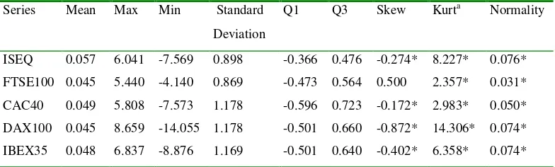
Summary Statistics are shown in table 1, where details of the first four moments,

the mean, standard deviation, skewness and centred kurtosis are presented.

Generally, these statistics show similar characteristics for the equity indexes,

namely, that daily returns on average are positive, risk levels are around one percent per day, there is excess negative skewness (FTSE100 excepted), and the returns are

leptokurtotic. This latter finding is the driving force behind the application of

extreme value theory and the assumption that the equity index returns are in the

maximum domain of attraction of the fat tailed, Fréchet distribution. Also, both

third and fourth moment values are evidence against the normal distribution at

Smirnov test Normality is formally examined with the

Kolmogorov-Smirnov test indicating that none of the indexes support the hypothesis of

belonging to a gaussian distribution. These findings are similar to previous studies

on equity markets. This non-normality suggests the ruling out of the mean-variance

framework applied in portfolio theory as a method of measuring the downside risk

estimates. In fact assuming normality results in an underestimation of tail

behaviour and by extension the associated downside risk measures. As this study

concentrates on extreme values for the downside risk measures statistics are also given for maximum and minimum values, as well as the first and third quantiles.

Again the indexes show similar values for the period analysed, of which the

DAX100 outliers shows the greatest range, and CAC40 has the largest interquartile

range. Notwithstanding the findings in table 1 however, these summary statistics

indicate that further analysis is required to get realistic outcomes on the downside

risk exposures facing investors on these exchanges.

INSERT TABLE 1 HERE

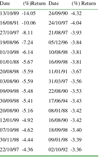
It is interesting to investigate further the more extreme downside return values

given the findings in table 1. Taking the DAX100 index as a case study (as this

portfolio experiences the greatest magnitude of losses), the lowest one percent of equity returns and their time of occurrence are presented in table 2. The beginning

and end of the sample period represent the highest negative extreme returns with

very few observations during the middle of the period of analysis. The extent of the

magnitude of the losses suffered in Frankfurt is evident by noting that the worst

sixteen returns in table 2 dominate the worst recorded return on the London

unlike the general findings from the analysis of the full distribution of financial

return datasets.

IV EMPIRICAL FINDINGS

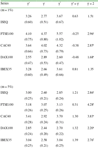
Empirical findings of the Hill tail index for each equity index are now discussed.

The lower tail estimates are given in table 3 for two threshold values of one and five percent, both in the spirit of the DuMouchel (1983) technique, but also

corresponding to the most commonly cited confidence levels. There are a number of interesting findings. To begin, the tail index values range from 2.44 (DAX100)

to 5.57 (FTSE100) for the analysis of all tail estimates. Concentrating specifically

on the downside tail estimates we see that the upper tail estimate is 4.37

(FTSE100). These values correspond to the general conclusions made for time

series of financial returns, namely that they have fat-tail characteristics. The

goodness of fit of each equity index being associated with the Fréchet distribution is

confirmed in table 2 using a difference in means statistic given in Koedijk and Kool

(1992). Specifically all tail values are significantly positive, corresponding to the

requirement that γ = α-1 > 0.

Previous studies on financial returns have classified the data according to different

fat-tailed distributions on the basis of the tail estimates obtained. We can

characterise Hill estimates with a value less than or equal to two as belonging to a

stable paretian family of distributions, whereas, for values greater than two, they

belong to GARCH related specifications (Ghose and Kroner, 1995). Formally, this

including belonging to the stable paretian family of distributions (Ho: γ- < 2), and

having GARCH characteristics (Ho: γ- > 2). Conclusions from the downside tail

estimates indicate that there is support for the stable paretian hypothesis being

rejected for all of the equities with the exception of the ISEQ and IBEX35 indexes

as the null (Ho: γ- < 2) is statistically rejected. In contrast, the indication that the tail

returns have GARCH features is never rejected.

INSERT TABLE 3 HERE

The tail estimates generally decrease as you move away from the one percent

threshold with the exception of the DAX100 index. Decreases in the estimates as

you move towards the centre of the distribution reaffirms the idea that the most

extreme returns have different distributional characteristics than the full sequence

of returns as suggested in the earlier data description. Although the main

discussion of this paper is on downside risk encompassing a long position, it is easy to extend the analysis to determine upside risk focusing on a short position, and a

common position regardless of the source of risk. In table 3, upside, γ+, and

common, γ*, tail estimates are presented. Using Loretan and Phillips (1994)

stability test we can conclude that our inferences on the VARq and ELp estimates

are equally appropriate for a short position with all lower tail estimates

insignificantly different from upper tail measures.

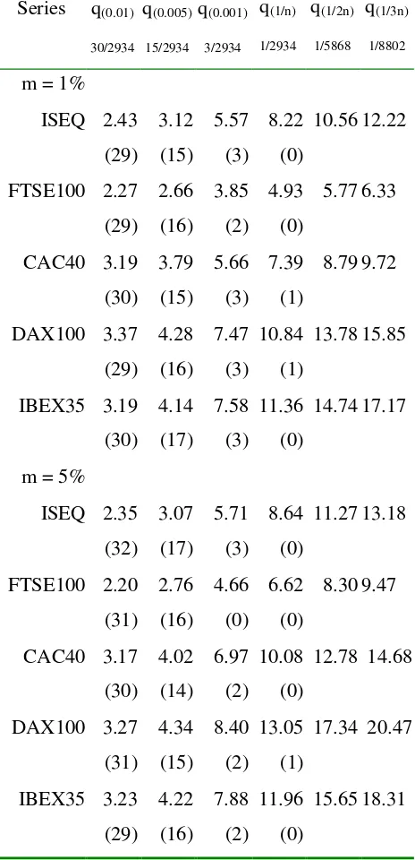
Turning to the VaR quantiles in table 4 both in-sample and out-of-sample estimates

are examined. For the two thresholds, m, we examine six probability levels, either

or 1 in 5868 (q(1/2n)), or 1 in 8802 (q(1/3n)), representing the expected number of

occurrences. The latter two probability levels represent out-of-sample estimates

detailing over 22 years and 33 years of return observations. These estimates could

not be obtained using the empirical distribution as we could only deal with

probabilities of 1/n or larger. However, extreme value theory allows for

semi-parametric estimation so very rare events outside of the sample size under analysis

can be examined. Hence, these VaR quantile estimates could not be obtained using

methods such as historical simulation due to a lack of data.6 The VaR quantiles are easy to interpret, for instance there is a 99 percent confidence that the downside risk

for the ISEQ index is less than or equal to 2.43% with a tail threshold, m, of 1%.

Losses in excess of this value would occur with a frequency of 1 in 100 days (n =

1/p) on average. The robustness of the VaR values is verified using the technique

outlined in Danielsson and de Vries (2000) comparing estimated to expected

occurrences.

INSERT TABLE 4 HERE

To begin, we see that the indexes exhibit reasonably similar tail volatility for high

probability levels with DAX100 exhibiting the highest (3.37% and 3.27%) VaR

quantiles for both thresholds in comparison to the FTSE100 exhibiting the lowest (2.27% and 2.20%) VaR quantiles.7 However, by moving out the tail to more

extreme quantiles we find two notable differences, namely, that the levels of

volatility increase substantially and that these increases in tail volatility become

dissimilar across stock indexes. On the former issue for instance, we see that the

in-sample to out-of-in-sample estimates. This is to be expected given the movement

further out the tail to more volatile returns. Whereas on the latter issue, the

out-of-sample estimates vary substantially at the tail threshold, m, of 5% (the variation

becomes even more pronounced for the 1% tail threshold, m) with the DAX100

now exhibiting downside risk of less than or equal to 15.85% in comparison to

6.33% for the FTSE100. This provides an insight into the respective volatility of

each individual index that would not normally be presented with more commonly

used statistical measures.

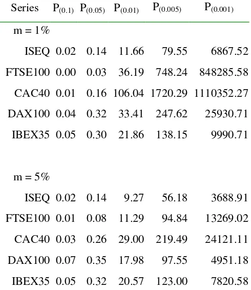
The excess loss probability estimators are presented in table 5 where both in-sample

and out-of-sample estimates are examined. Again we examine two thresholds, and

provide a large number of extreme value estimates for the downside risk of the

European indexes. Five percentage quantiles are presented and we determine the

probability of each index exhibiting the sufficient volatility to be in excess of these

quantiles. These quantiles are (negative) 10% (P(0.1)), 5% (P(0.05)), 1% (P(0.01)), 0.5%

(P(0.005)), and 0.1% (P(0.001)). The excess loss probability estimators imply that the

probability on any given day of having a negative return exceeding 10% for the

ISEQ index is 0.02% with a tail threshold, m, of 1%. Any value in excess of 100

relates to the out-of-sample occurrence of an event as we are certain that that

percentage quantile will be exceeded in the time frame analysed and would have a likelihood of occurrence in an extended time period.

As we can see in table 5, there is a very low probability of the respective indexes

exceeding large losses such as 10%. For instance, the most risky asset at this

quantile of the tail is the DAX100 index at the 1% threshold, m, with an associated

probability of 0.07%. However, as you move to smaller losses, the associated

probability levels increase as expected a priori that this negative relationship

occurs. To illustrate, we see that there is a 100% likelihood that each index will

incur losses in excess of 0.1%. Obviously such price movements are minimal in the

context of observed daily volatility for risky assets such as equities and these are expected to definitely occur. Returning to larger losses such as 1%, we see for

example that there is a 36.19% probability of downside returns being in excess of

this loss level for the FTSE100 index. This can be measured in terms of the actual

numbers of days (given the sample size) that the London traded index exceeds these

loss levels with occurrences of 1062 days as given by the calculation n*p.

As stated the DAX100 index exhibits the most volatility around the very large loss

levels such as 10% or even 5%. However as you move to more common (or

smaller) loss levels we see that the other indexes indicate more volatility, with for

example both the FTSE100 and CAC40 indexes having a greater probability of

exceeding losses of 0.1% at the 1% threshold, m. The rational for this divergence

at different loss levels can be explained in terms of relative fatness of the tail and the relative scale of the tail values. Generally, we can conclude that the FTSE100

and CAC40 index have fatter tails than the DAX100 index with their higher

propensity to exceed the lower loss levels. In comparison the relatively thin tailed

DAX100 contract at these lower loss levels has extreme values of greater

in the second column of table 5. Further evidence supporting this rational can be

found in terms of the magnitude of the extreme values for this index presented in

table 4 for all VaR quantiles and in table 2 with the largest minimum value.

V CONCLUSIONS

This paper applies extreme value theory to measure downside risk for European

equity markets. Two related risk measures are presented, the popular Value at Risk

estimator, and the Excess Loss probability estimator. Overall, these measures allow

for a coherent risk management approach to optimally protect investor wealth

opportunities. Given the large fluctuations inherent in equity markets, the empirical

application examines combinations of low quantile and probability estimates.

Whilst these downside events may not occur with everyday regularity, their

consequences demand a thorough analysis. Fortunately, the extreme value approach focuses on tail price fluctuations at the expense of the whole distribution,

as it is these outcomes that affect the relative ability for an investor’s portfolio to survive in the face of large price movements.

Extreme value theory dominates alternative approaches in tail estimation as it

avoids model risk. Alternative approaches such as the variance covariance and

Monte Carlo methods model the full distribution of returns, whereas this study’s

focus of attention, the tail values are explicitly modelled by extreme value theory.

Also, extreme value theory operates on the basis that the regular variation at infinity

exactly match any set of returns exhibiting a fat-tailed characteristic with a

particular distributional form. Moreover, the theoretical approach adopted here

advantageously can be extended for different frequencies and for out-of-sample

estimates using parsimonious techniques. The former relies on a simple scaling law

whereas the latter exploits the semi-parametric estimation technique to extend

beyond a given sample size. On the issue of semi-parametric estimation, the paper

utilises the moments based Hill estimator, which dominates other tail estimators on

bias and efficiency grounds.

Notwithstanding the agreement with general findings of excess skewness,

leptokurtosis and a lack of normality cited for equity markets, this paper makes a

number of interesting findings. First, all equity series’ statistically belong to the

Fréchet distribution, and more specifically exhibit GARCH characteristics at the

expense of the stable paretian model. Second, whereas the VaR quantiles increase

from in-sample to out-of-sample estimates, the degree of these increases vary

according to each index. In particular, the DAX100 index exhibits comparably

higher downside risk levels demonstrating this portfolio’s unique volatility pattern

identified by extreme value analysis. Third, the excess probability estimates

provide further evidence of the implications of the respective fat-tailed characteristics of each index. Here, we find that the FTSE100 and CAC40 indexes

differ from the DAX100 series in that they have a higher propensity for exceeding

relatively small losses but a lower propensity for exceeding relatively large losses.

Finally, we conclude that all our inferences on the downside VaR quantile and

excess probability estimates hold for the upside due to the stability of returns

ACKNOWLEDGEMENTS

The author would like to thank participants at the Economics Department seminar,

University College Cork for their helpful comments on this paper. Financial

REFERENCES

Artzner, P., DelBaen, F., Eber, J. and Heath, D. (1999) Coherent measures of risk,

Mathematical Finance, 8, 203-228.

Arzac, E. R., and Bawa, V. S. (1977) Portfolio choice and equilibrium in capital

markets with safety-first investors, Journal of Financial Economics, 4, 277-288.

Cotter, J. (2001) Margin exceedences for european stock index futures using extreme value theory, Journal of Banking and Finance, 25, 1475-1502.

Danielsson, J and DeVries, C. G. (1997a) Tail index and quantile estimation with very high frequency data, Journal of Empirical Finance, 4, 241-257.

Danielsson, J and DeVries, C. G. (1997b) Beyond the sample: extreme quantile and

probability estimation, Mimeo, Timbergen Institute Rotterdam, December.

Danielsson, J and DeVries, C. G. (2000) Value at Risk and extreme returns,

Annales D’Economie et de Statistique, 60, 239-270.

Diebold, F. X., Schuermann, T. and Stroughair, J. D. (1998) Pitfalls and

opportunities in the use of extreme value theory in risk management, in Advances in

Computational Finance, (Editors) J. D. Moody and A. N. Burgess, Kluwer,

Amsterdam.

Duffie, D., and Pan, J. (1997) An overview of value at risk, Journal of Derivatives,

4, 7-49.

Feller, W. (1971) An introduction to probability theory and its applications, John

Wiley, New York.

Gallagher, L. A. (1999) A multi-country analysis of the temporary and permanent

Ghose, D., and Kroner, K. F. (1995), The relationship between garch and

symmetric stable processes: finding the source of fat tails in financial data, Journal

of Empirical Finance, 2. 225-251.

Hill, B. M. (1975) A simple general approach to inference about the tail of a

distribution, Annals of Statistics, 3, 1163-1174.

Jansen, D. W., Koedijk, K. G. and DeVries, C. G. (2000) Portfolio selection with limited downside risk, Journal of Empirical Finance, 7, 247-269.

Kearns, P. and Pagan, A. (1997) Estimating the density tail index for financial time series, The Review of Economics and Statistics, 79, 171-175.

Koedijk, K. G. and Kool, C. J. M. (1992) Tail estimates of east european exchange

rates, Journal of Business and Economic Statistics, 10, 83-96.

Leadbetter, M. R., Lindgren, G. and Rootzen, H. (1983) Extremes and related

properties of random sequences and processes, Springer, New York.

Loretan, M. and Phillips, P. C. B. (1994) Testing the covariance stationarity of

heavy-tailed time series, Journal of Empirical Finance, 1, 211-248.

Poon, S. H., and Taylor, S. (1992) Stock returns and volatility: an empirical study

of the UK stock market, Journal of Banking and Finance, 45, 37-59.

Venkataraman, S. (1997) Value at Risk for a mixture of normal distributions: the use of quasi-bayesian estimation techniques, Federal Reserve Bank of Chicago's

Figure 1: Value at Risk for a downside quantile of the distribution of returns

F(R)

1

q

Figure 2: Left tail of fat-tailed and normal distribution

Table 1: Summary Statistics of Equity Index Returns

Series Mean Max Min Standard Deviation

Q1 Q3 Skew Kurta Normality

ISEQ 0.057 6.041 -7.569 0.898 -0.366 0.476 -0.274* 8.227* 0.076* FTSE100 0.045 5.440 -4.140 0.869 -0.473 0.564 0.500 2.357* 0.031* CAC40 0.049 5.808 -7.573 1.178 -0.596 0.723 -0.172* 2.983* 0.050* DAX100 0.045 8.659 -14.055 1.178 -0.501 0.660 -0.872* 14.306* 0.074* IBEX35 0.048 6.837 -8.876 1.169 -0.501 0.640 -0.402* 6.358* 0.074*

Table 2: Dates and Lowest One Percent Extreme Values for DAX100 index Returns

Table 3: Tail Index Estimates for European Stock Indexes

Series γ+ γ- γ* γ+ = γ- γ- = 2 (m = 1%)

ISEQ 3.26 (0.60) 2.77 (0.51) 3.67 (0.67)

0.63 1.51

FTSE100 4.10 (0.75)

4.37 (0.80)

5.57 (1.02)

-0.25 2.96•

CAC40 3.64 (0.66)

4.02 (0.73)

4.32 (0.79)

-0.38 2.85•

DAX100 2.55 (0.47)

2.89 (0.53)

2.60 (0.47)

-0.48 1.68•

IBEX35 3.28 (0.60)

2.66 (0.49)

3.61 (0.66)

0.81 1.35

(m = 5%)

ISEQ 3.00 (0.25)

2.60 (0.21)

2.85 (0.24)

1.21 2.86•

FTSE100 3.18 (0.26)

3.07 (0.25)

3.13 (0.26)

0.31 4.28•

CAC40 3.41 (0.28)

2.92 (0.24)

3.70 (0.31)

1.30 3.83•

DAX100 2.85 (0.24)

2.44 (0.20)

2.70 (0.22)

1.32 2.20•

IBEX35 3.04 (0.25)

2.58 (0.21)

3.04 (0.25)

1.39 2.76•

Table 4: Quantile Estimates for European Stock Indexes Series q(0.01)

30/2934 q(0.005) 15/2934 q(0.001) 3/2934 q(1/n) 1/2934 q(1/2n) 1/5868 q(1/3n) 1/8802

m = 1%

ISEQ 2.43 (29) 3.12 (15) 5.57 (3) 8.22 (0)

10.56 12.22

FTSE100 2.27 (29) 2.66 (16) 3.85 (2) 4.93 (0)

5.77 6.33

CAC40 3.19 (30) 3.79 (15) 5.66 (3) 7.39 (1)

8.79 9.72

DAX100 3.37 (29) 4.28 (16) 7.47 (3) 10.84 (1)

13.78 15.85

IBEX35 3.19 (30) 4.14 (17) 7.58 (3) 11.36 (0)

14.74 17.17

m = 5% ISEQ 2.35 (32) 3.07 (17) 5.71 (3) 8.64 (0)

11.27 13.18

FTSE100 2.20 (31) 2.76 (16) 4.66 (0) 6.62 (0)

8.30 9.47

CAC40 3.17 (30) 4.02 (14) 6.97 (2) 10.08 (0)

12.78 14.68

DAX100 3.27 (31) 4.34 (15) 8.40 (2) 13.05 (1)

17.34 20.47

IBEX35 3.23 (29) 4.22 (16) 7.88 (2) 11.96 (0)

15.65 18.31

The values in this table represent the VaR quantiles for different confidence intervals, for example q(0.01) is the 1% level. The estimates are based on different

threshold values, m, which are used to calculate the associated lower tail estimates,

Table 5: Probability Estimates for European Stock Indexes Series P(0.1) P(0.05) P(0.01) P(0.005) P(0.001)

m = 1%

ISEQ 0.02 0.14 11.66 79.55 6867.52 FTSE100 0.00 0.03 36.19 748.24 848285.58 CAC40 0.01 0.16 106.04 1720.29 1110352.27 DAX100 0.04 0.32 33.41 247.62 25930.71 IBEX35 0.05 0.30 21.86 138.15 9990.71

m = 5%

ISEQ 0.02 0.14 9.27 56.18 3688.91 FTSE100 0.01 0.08 11.29 94.84 13269.02 CAC40 0.03 0.26 29.00 219.49 24121.11 DAX100 0.07 0.35 17.98 97.55 4951.18 IBEX35 0.05 0.32 20.57 123.00 7820.58

The values in this table represent the probability of returns exceeding a certain threshold, for example, P(0.1) is 10 percent on any single day. The estimates are

FOOTNOTES

1 This paper exclusively analyses downside risk, the outcomes of interest for a long

position located at the left tail of the distribution of stock index returns. The theory

utilised is equally applicable for a short position dealing with the right tail of a

distribution.

1 VaR was originally developed as part of the Riskmetrics system produced by JP

Morgan to meet the requirement of its CEO Dennis Weatherstone to have a single

measure of risk exposure presented to him on a daily basis. The measure has quickly spread to become a mainstream and commonly used risk management

analytical tool. However, downside quantile estimation has been applied in the past

prior to the J.P.Morgan development (see Arzac and Bawa, 1977; for one such

illustration of portfolio selection with an inbuilt safety criteria).

3 There may also be a regulatory need to have VaR measures over longer periods,

for example, the Basle capital requirements for a ten day holding period.

4 The maximum domain of attraction does not operate in reverse, so the assumption

that the mixtures of normals converges to a Fréchet distribution does not imply that

the Fréchet reaslisations follow a mixtures of normals process.

5 Whilst it is recognised that an investor's diversified portfolio may not actually

match any of the indexes analysed, they are representative of diversified groups of individual equities traded on the respective exchanges.

6 Using historical simulation would accentuate the problem even further if the

returns series was smaller (common in many academic studies).

7 The effects of German unification are an obvious cause of these high volatility

example industry sector analysis, may provide further indications of the source of