Improved Quantum Behaved Particle Swarm Optimization

http://dx.doi.org/10.4236/ojapps.2015.56025

Improved Quantum-Behaved Particle

Swarm Optimization

Jianping Li

School of Computer and Information Technology, Northeast Petroleum University, Daqing, China

Email: [email protected]

Received 23 April 2015; accepted 30 May 2015; published 2 June 2015

Copyright © 2015 by author and Scientific Research Publishing Inc.

This work is licensed under the Creative Commons Attribution International License (CC BY).

http://creativecommons.org/licenses/by/4.0/

Abstract

To enhance the performance of quantum-behaved PSO, some improvements are proposed. First, an encoding method based on the Bloch sphere is presented. In this method, each particle carries three groups of Bloch coordinates of qubits, and these coordinates are actually the approximate solutions. The particles are updated by rotating qubits about an axis on the Bloch sphere, which can simultaneously adjust two parameters of qubits, and can automatically achieve the best matching of two adjustments. The optimization process is employed in the n-dimensional space [-1, 1]n, so this approach fits to many optimization problems. The experimental results show that this algorithm is superior to the original quantum-behaved PSO.

Keywords

Swarm Intelligence, Particle Swarm Optimization, Quantum Potential Well, Encoding Method

1. Introduction

solutions to hard optimization problems. At present, the classical PSO method has been successfully applied to combinatorial optimization [2][3] and numerical optimization [4][5]. The following improvements have been applied to the classical PSO technique: modification of design parameters [6]-[8], modification of the update rule of a particle’s location and velocity [9][10], integration with other algorithms [11]-[17], and multiple sub- swarms PSO [18][19]. These improvements have enhanced the performance of the classical PSO in varying de-grees.

Quantum PSO (QPSO) is based on quantum mechanics. A quantum-inspired version of the classical PSO al-gorithm was first proposed in [20]. Later Sun et al. introduced the mean best position into the algorithm and proposed a new version of PSO, quantum-behaved particle swarm optimization [21][22]. The QPSO algorithm permits all particles to have a quantum behavior instead of the Newtonian dynamics of the classical PSO. In-stead of the Newtonian random walk, a quantum motion is used in the search process. The iterative equation of QPSO is very different from that of PSO, and the QPSO needs no velocity vectors for the particles. One of the most attractive features of the new algorithm is the reduced number of control parameters. Only one parameter must be tuned in QPSO, which makes it easier to implement. The QPSO algorithm has been shown to success-fully solve a wide range of continuous optimization problems and many efficient strategies have been proposed to improve the algorithm [23]-[27].

In order to enhance the optimization ability of QPSO by integrating quantum computation, we propose an improved quantum-behaved particle swarm optimization algorithm. In our algorithm, all particles are encoded by qubits described on the Bloch sphere. The three-dimensional Cartesian coordinates of qubits can be obtained from projective measurement. Since each qubit has three coordinate values, each particle has three locations. Each of the locations represents an optimization solution, which accelerates the search process by expanding the search scope of each variable from an interval on the number axis to an area of the Bloch sphere. The delta po-tential well is used to establish the search mechanism. Pauli matrices are used to perform the projective mea-surement, establish the rotation matrices and achieve qubits rotating about the rotation axis. The experimental results show that the proposed algorithm is superior to the original one in optimization ability.

2. The QPSO Model

In quantum mechanics, the dynamic behavior of a particle complies with the following Schrodinger equation

( )

_, 2 2

( ) ( )

_,

2

j r t V r r t

t m

 

∂ _{Ψ = − ∇ + Ψ}

 

∂ _{ }



 (1)

where  denotes Planck’s constant, m denotes particle quality and V(r) denotes the energy distribution func-tion.

In Schrodinger’s equation, the unknown is the wave function Ψ

( )

r t, . According to the statistical interpreta-tion of this wave funcinterpreta-tion, the square of its magnitude denotes the probability density. Taking the delta potential well as an example, the design of QPSO is described as follows.

The potential energy distribution function of the delta potential well can be expressed as

( )

( )

V r = −γδ r (2)

where γ denotes the potential well depth.

Substituting Equation (2) into Equation (1), we can obtain a particle’s wave function,

( )

1

e r L r

L −

Ψ = (3)

where

2

L mγ

=  denotes the characteristic length of the delta potential well.

Therefore, a particle’s probability density function can be written as

( )

( )

2 1 2

e r L

Q r r

L

−

= Ψ = (4)

( )

| d 0.5

r

rQ r r

− >

∫

(5)

From Equations (4) and (5), the characteristic length, L, must satisfy

( )

(

1

)

ln 2 r

L g

g

= > ₍₆₎

In the potential well, the dynamic behavior of the particles obeys the Schrodinger equation, in that the par-ticles’ locations are random at any time. However, the particles in classical PSO obey Newtonian mechanics, where the particles must have definite locations at any time. This contradiction can be satisfactorily resolved by means of the collapse of the wave function and the Monte Carlo method. We first take a random number u in the range (0,1) and let u=e−2r L, then the following result can be obtained

1 ln 2 L r

u

 

= _{ }

  (7)

Using Equations (6) and (7), we can derive that 1

( )

ln 1

2 ln 2

k k

u

r r

g

+ = . Let rk =xk−P. It is then possible to

de-rive 1

( )

ln 1

2 ln 2

k k

u

x P x P

g

+ = ± − . By letting 1

2 ln 2g

α = ,

( )

1 ln 1

k k

x₊ = ±P α x −P u (8)

The above formula is the iterative equation of QPSO [26][27].

3. The QPSO Improvement Based on Quantum Computing

In this section, we propose a Bloch sphere-based quantum-behaved particle swarm optimization algorithm called BQPSO.

3.1. The Spherical Description of Qubits

In quantum computing, a qubit is a two-level quantum system, described by a two-dimensional complex Hilbert space. From the superposition principles, any state of the qubit may be written as

( )

( )

cos θ 2 0 e siniϕ θ 2 1

= +

ϕ (9)

where 0≤ ≤θ π, 0≤ ≤φ 2π.

Therefore, unlike the classical bit, which can only equal 0 or 1, the qubit resides in a vector space paramete-rized by the continuous variables θ and ϕ. The normalization condition means that the qubit’s state can be represented by a point on a sphere of unit radius, called the Bloch sphere. The Bloch sphere representation is useful as it provides a geometric picture of the qubit and of the transformations that can be applied to its state. This sphere can be embedded in a three-dimensional space of Cartesian coordinates (x=cos sinϕ θ, y=sin sinϕ θ,

cos

z= θ). Thus, the state ϕ can be written as

(

)

T

1 i

,

2 2 1

z x y

z

 _{+ +} 

 

=

 + 

 

ϕ (10)

The optimization is performed in

[

−1, 1

]

n, so the proposed method can be easily adapted to a variety of opti-mization problems.

3.2. The BQPSO Encoding Method

1 , 2 , ,

i i i in

p = φ φ  φ _ (11)

where

T i

cos , e sin ; 0 π; 0 2π; 1, 2, , ; 1, 2, , .

2 2

ij ij

ij ij ij i m j n

ϕ

θ θ

φ =_ _ ≤θ ≤ ≤ϕ ≤ = =

   

From the principles of quantum computing, the coordinates x, y, and z of a qubit on the Bloch sphere can be measured by the Pauli operators written as

0 1 0 i 1 0

, ,

1 0 i 0 0 1

x y z

−

     

=_{ } =_{ } =_{ }

−

     

σ σ σ (12)

Let φij denote the j-th qubit on the i-th particle. The coordinates (xij, yij, zij) of φij can be obtained by

Pauli operators using

0 1

1 0

ij ij x ij ij ij

x = = _ _

 

ϕ σ ϕ ϕ ϕ (13)

0 i

i 0

ij ij y ij ij ij

y = = _ −_

 

ϕ σ ϕ ϕ ϕ (14)

1 0

0 1

ij ij z ij ij ij

z = = _ _

−

 

ϕ σ ϕ ϕ ϕ (15)

In BQPSO, the Bloch coordinates of each qubit are regarded as three paratactic location components, each particle contains three paratactic locations, and each location represents an optimization solution. Therefore, in the unit space

[

−1, 1

]

n, each particle simultaneously represents three optimization solutions, which can be de-scribed as follows

[

]

[

]

[

]

1 2

1 2

1 2

, , ,

, , ,

, , ,

ix i i in

iy i i in

iz i i in

p x x x

p y y y

p z z z

 =

 ₌



 ₌



  

(15)

3.3. Solution Space Transformation

In BQPSO, each particle contains 3n Bloch coordinates of n qubits that can be transformed from the unit space

[

−1, 1

]

n to the solution space of the optimization problem. Each of the Bloch coordinates corresponds to an op-timization variable in the solution space. Let the j-th variable of optimization problem be Xj∈ A Bj, j, and

(

x_ij,y_ij,z_ij

)

denote the coordinates of the j-th qubit on the i-th particle. Then the corresponding variables

(

X_ij,Y Z_ij, _ij

)

in the solution space are computed as follows

(

1

)

(

1

)

2

ij j ij j ij

X =_B −x +A +x _ (16)

(

1

)

(

1

)

2

ij j ij j ij

Y =_B −y +A +y _ (17)

(

1

)

(

1

)

2

ij j ij j ij

Z =_B −z +A +z _ (18)

where i=1, 2,,m j; =1, 2,, .n

3.4. The Optimal Solutions Update

By substituting the three solutions

[

Xi1,,Xin

] [

, Yi1,,Yin

] [

, Zi1,,Zin

]

described by the i-th particle into the fitness function, we may compute its fitness, for i=1, 2,,m. Let gfitbest denote the best fitness so far, and

best

denote the corresponding best particle. Further, let fit p

( )

i =max

(

fit X Y Z

(

i, ,i i

)

)

,

(

( )

)

1

max best

i m

fit fit p i

≤ ≤

= . If

( )

(

( )

)

cfit i < fit p i then cfit i

( )

= fit p i

(

( )

)

and cpi = pi . If gfitbest < fit best

(

)

then gfitbest = fit best

(

)

and gpbest = pbest.

3.5. Particle Locations Update

In BQPSO, we search on the Bloch sphere. That is, we rotate the qubit around an axis towards the target qubit. This rotation can simultaneously change two parameters θ and ϕ of a qubit, which simulates quantum beha-vior and enhances the optimization ability.

For the i-th particle, let Pij denote the current location of the j-th qubit φij on the Bloch sphere, and

L ij P and Pgj denote its own best location and the global best location on the Bloch sphere. According to [27], for

ij

P _{, the two potential well centers in Equation (8) can be obtained using}

( )

1

1

m L ij

c i

ij m L

ij i P m P k P m = = =

∑

∑

(19)

(

)

(

)

(

)

1 1 1 L ij gj c ij _L ij gj

rP r P

P k

rP r P

+ − + =

+ − (20)

where m denotes the number of particles, r denotes a random number uniformly distributed in (0, 1), and k de-notes the iterative step.

Let O denote the center of the Bloch sphere and βij

( )

k denote the angle between OPij and

( )

c ij k

OP .

From the QPSO’s iteration equation, to make Pij move to

(

1

)

c ij

P k+ , the angle β_ij

(

k+1

)

needs to be ro-tated on the Bloch sphere so that

(

1

)

ln 1

( ) ( ) (

, 0 1

)

ij k u ij k

β + = ±α β <α< (21)

Let the qubit corresponding to the point c

(

1

)

ij

P k+ be φijc . From the above equation we know that the new

location of φij is actually the location of c ij

φ after it is rotated through an angle β_ij

(

k+1

)

towards φij .

To achieve this rotation, it is crucial to determine the rotation axis, as it can directly impact the convergence speed and efficiency of algorithm. According to the definition of the vector product, the rotation axis of rotating

c ij

φ towards φij through an angle βij

(

k+1

)

can be written as

(

)

( )

(

)

( )

1 1 c ij ij axis _c ij ij k k k k + × = + × OP OP R

OP OP (22)

From the principles of quantum computing, the rotation matrix about the axis Raxis that rotates the current qubit φij towards the target qubit

c ij

φ _{can be written as}

( )

(

)

cos

( )

isin

( ) (

)

2 2

ij ij

ij axis

k k

M β k = β I− β R ×σ (23)

and the rotation operation can be written as

(

1

)

(

(

1

)

)

c

( )

ij k M ij k ij k

φ + = β + φ (24)

where i=1, 2,, ,m j=1, 2,, ,n and k denotes the iterative steps.

4. Experimental Results and Analysis

4.1. Test Functions

1) 1

( )

11

(

100

(

1 2

)

2

(

1

)

2

)

D

i i i

i

f X =

∑

=− x+ −x + x − ;

2) 8

( )

1

( )

1

418.9828872724338 D _isin _i

i

f X x x

D =

= −

∑

;

3) 13

( )

(

)(

)

1

(

)

2 2 1

4 1

1 6

D D

i i i

i i

D D D

f X = x = x x−

+ −

= +

∑

− −

∑

;

4)

( )

( )

2 20

16 1sin sin π

D _i

i i

ix f X = − ₌ x _ _

 

∑

;

5)

( )

( )

2

18 1 1 ₄₀₀₀ cos , 1

D D jk

j k k j

y

f X = _{= =}_ − y + _

 

∑ ∑

,

(

2

)

2

(

)

2

100 1

jk k j j

y = x −x + −x ;

6) 19

( )

14

(

(

4 3 10 4 2

)

2 5

(

4 1 4

) (

2 4 2 2 4 1

)

4 10

(

4 3 4

)

4

)

D

i i i i i i i i

i

f X =

∑

₌ x ₋ + x ₋ + x ₋ −x + x ₋ − x ₋ + x ₋ −x ;

7) 21

( )

10 1

(

2 10 cos 2π

(

)

)

D

i i

i

f X = D+

∑

₌ y − y ,

( )

, 1 2

2 2 , 1 2

i i

i

i i

x x

y

round x x

 <

 = 

≥

 ;

8) 22

( )

1

{

max0 cos 2

(

π

(

0.5

)

)

}

max0

(

cos

( )

π

)

D k k k k k k

i

i k k

f X =

∑ ∑

_{= =} _a b x + _ −D

∑

₌ a b .

4.2. Experimental Setup

For all problems, the following parameters are used unless a change is mentioned. Population size: NP = 100 when D = 30 and NP = 80 when D = 20, the precision of a desired solution value to reach (VTR): VTR = 10 − 5

(i.e. f X

( )

f X

(

optimal

)

105 −

− < ) for f1 and f6; VTR = 100 for f2 and f5; VTR = 0.1 for f3; VTR = 10

for f4 and f7; VTR = 0.001 for f8. The maximum of the number of function evaluations (MNFE): MNFE =

20000; The control parameter: α =0.8; Halting criterion: when MNFE is reached, the execution of the algo-rithm is stopped.

To minimize the effect of the stochastic nature of the algorithms, 50 independent runs on 8 functions are per-formed and the reported indexes for each function are the average over 50 trials. If an algorithm finds the global minima with predefined precision within the preset MNFE the algorithm is said to have succeeded. Otherwise it fails. All of the algorithms were implemented in standard Matlab 7.0 and the experiments were executed on a P-II 2.0 GHz machine with 1.0 GB RAM, under the WIN-XP platform.

4.3. Performance Criteria

Five performance criteria were selected from [31] to evaluate the performance of the algorithms. These criteria are also used in [32] and are described as follows.

Error: The error of a solution X is defined as f X

( )

− f X

( )

* , where *

X is the global optimum of the function. The error was recorded when the MNFE was reached and the average (mean) and standard deviation (std dev) of the 50 error values were calculated.

NFE: When the VTR was reached, the number of function evaluations (NFE) was recorded. If the VTR was not reached within the preset MNFE then the NFE is equal to MNFE. The average (mean) and standard devia-tion (std dev) of the 50 NFE values were calculated.

Number of successful runs (SR): The number of successful runs was recorded when the VTR was reached before the MNFE was satisfied.

Running time (time (s)): Running time indicates the average time over one function evaluation.

4.4. Comparison Results

BQPSO. The parameters used for the two algorithms are described in Section 4.2. The results were calculated using 50 independent runs. Table 1 shows the mean and standard deviation of the errors of BQPSO and QPSO on 8 benchmark functions. The mean and standard deviation of NFE are shown in Table 2.

From Table 1 and Table 2, we can see that BQPSO performs significantly better than QPSO for 8 functions. For f2, f4, f6, BQPSO succeed in finding the minimum in all runs. For the other functions, BQPSO succeed

[image:7.595.94.539.182.444.2]

much more often than QPSO. Furthermore, BQPSO obtains smaller mean and standard deviations than QPSO

Table 1.Comparison of the mean and standard deviation of the error of BQPSO and QPSO on 8 benchmark functions.

F D MNFE BQPSO QPSO

Mean Std dev SR Time (s) mean Std dev SR Time (s) f1 30 20,000 0.079 73 0.317 86 49 0.037 47 23.0011 452.679 1 0.00184

20 20,000 0.239 19 0.914 67 47 0.016 71 3.01441 7.96305 6 0.00155 f2 30 20,000 38.9119 503.099 50 0.037 11 222.619 206.335 0 0.00263

20 20,000 28.2399 331.000 50 0.016 35 120.592 3215.47 11 0.00170 f3 30 20,000 0.089 91 0.039 48 40 0.037 43 621.143 178731.2 0 0.00242

20 20,000 2.9E−09 1.1E−18 50 0.016 46 8.49475 81.7811 4 0.00179 f4 30 20,000 −28.169 0.322 38 50 0.031 39 −10.971 0.57122 0 0.00485

20 20,000 −18.866 0.180 42 50 0.016 60 −9.1920 0.43015 15 0.00270 f5 30 20,000 141.237 70671.1 37 0.053 73 260.084 7081.92 3 0.01753

20 20,000 31.1062 935.123 48 0.029 56 102.068 1255.77 21 0.00709 f6 32 20,000 1.3E−07 1.0E−15 50 0.033 22 3.9E−04 4.0E−08 0 0.00316

24 20,000 3.8E−08 8.7E−17 50 0.016 64 7.0E−05 1.8E−09 4 0.00236 f7 30 20,000 7.680 00 10.8751 36 0.036 97 21.9300 57.9156 0 0.00296

20 20,000 4.020 00 3.203 67 50 0.016 67 8.33940 6.03014 37 0.00222 f8 30 20,000 0.324 16 0.454 06 30 0.446 92 28.6777 5.51655 0 0.03800

[image:7.595.92.539.469.723.2]

20 20,000 0.100 63 0.164 75 46 0.267 24 14.4137 2.11969 0 0.02871

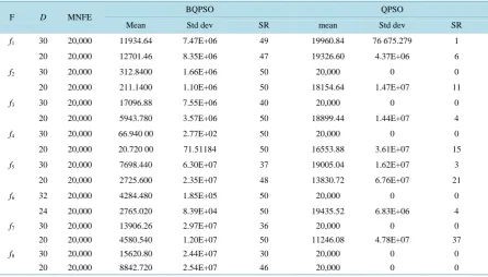
Table 2.Comparison of the mean and standard deviation of the NFE of BQPSO and QPSO on 8 benchmark functions.

F D MNFE BQPSO QPSO

Mean Std dev SR mean Std dev SR

f1 30 20,000 11934.64 7.47E+06 49 19960.84 76 675.279 1

20 20,000 12701.46 8.35E+06 47 19326.60 4.37E+06 6

f2 30 20,000 312.8400 1.66E+06 50 20,000 0 0

20 20,000 211.1400 1.10E+06 50 18154.64 1.47E+07 11

f3 30 20,000 17096.88 7.55E+06 40 20,000 0 0

20 20,000 5943.780 3.57E+06 50 18899.44 1.44E+07 4

f4 30 20,000 66.940 00 2.77E+02 50 20,000 0 0

20 20,000 20.720 00 71.51184 50 16553.88 3.61E+07 15 f5 30 20,000 7698.440 6.30E+07 37 19005.04 1.62E+07 3

20 20,000 2725.600 2.35E+07 48 13830.72 6.76E+07 21

f6 32 20,000 4284.480 1.85E+05 50 20,000 0 0

24 20,000 2765.020 8.39E+04 50 19435.52 6.83E+06 4

f7 30 20,000 13906.26 2.97E+07 36 20,000 0 0

20 20,000 4580.540 1.20E+07 50 11246.08 4.78E+07 37

f8 30 20,000 15620.80 2.44E+07 30 20,000 0 0

for 8 functions. Especially, for f2

(

D=30

)

, f3

(

D=30

)

, f4

(

D=30

)

, f6

(

D=30

)

, f7

(

D=30

)

, and

(

)

8 30

f D= , BQPSO succeeds many times while all runs of QPSO fail. In Table 1, we can see that there are significant differences in quality between the BQPSO and QPSO solutions of the high-dimensional functions.

In Table 2, the MNFE is fixed at 20000 for 8 functions. From this table it can be observed that, for all func-tions, BQPSO requires less NFE than QPSO. For some high-dimensional functions (such as f2

(

D=30

)

,

(

)

3 30

f D= , f4

(

D=30

)

, f6

(

D=30

)

, f7

(

D=30

)

and f8, QPSO fails to reach the VTR after 20,000

NFE while BQPSO is successful. It is worth noting that, from Table 1, the running time of BQPSO is about 10 to 20 times longer than that of QPSO. According to the no free lunch theorem, the superior performance of BQPSO is at the expense of a long running time.

It can be concluded that the overall performance of BQPSO is better than that of QPSO for all 8 functions. The improvement based on quantum computing can accelerate the classical QPSO algorithm and significantly reduce the NFE to reach the VTR for all of the test functions.

4.5. The Comparison of BQPSO with Other Algorithms

In this subsection, we compare BQPSO with other state-of-art algorithms to demonstrate its accuracy and per-formance. These algorithms include a genetic algorithm with elitist strategy (called GA), a differential evolution algorithm (called DE), and a bee colony algorithm (called BC). The BQPSO’s control parameter was α =0.8. For the genetic algorithm, the crossover probability was Pc =0.8 and the mutation probability was Pm =0.05. For the differential evolution algorithm, the scaling factor was λ = =F 0.6, and the crossover probability was

0.8

CR= . For the bee colony algorithm, let N denote the population size of the whole bee colony, and Ne and Nu denote the population size of the employed bee and onlooker bee, respectively.

We have taken Ne=Nu. The threshold of a tracking bee searching around a mining bee was Limit=100. The other parameters used for the four algorithms are the same as described in Section 4.2. The eight high-dimensional functions were used for these experiments, which had 50 independent runs. Table 3 shows the mean of these 50 errors and the number of successful runs. The mean and standard deviation of the NFE are shown in Table 4.

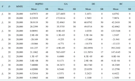
[image:8.595.88.539.452.722.2]

From Table 3 and Table 4 it can be argued that the BQPSO performed best among the four algorithms. It ob-tained the best results for all eight benchmark functions. The best algorithm is not as obvious for the remaining

Table 3.Comparison of the mean of the error and the number of successful runs of the four algorithms.

F D MNFE

BQPSO GA DE BC

Mean SR Mean SR Mean SR Mean SR

f1 30 20,000 0.07973 49 227.4855 0 3.1071 0 6.0792 0

20 20,000 0.23919 47 172.8114 0 1.7693 0 7.9874 0 f2 30 20,000 38.9119 50 52.4963 50 60.8792 50 42.2418 50

20 20,000 28.2399 50 35.5755 50 49.0714 50 42.6962 50 f3 30 20,000 0.08991 40 8.9E+03 0 1.0330 10 125.5168 0

20 20,000 2.9E–09 50 1.3E+03 0 3.3E−04 50 1.5107 3 f4 30 20,000 –28.169 50 –9.255 0 –17.060 0 –21.941 45

20 20,000 –18.866 50 –6.771 0 –14.574 0 –13.133 0 f5 30 20,000 141.237 37 4.9E+05 0 282.0958 3 393.2102 18

20 20,000 31.1062 48 765.4107 4 111.5074 17 147.4145 34 f6 32 20,000 1.3E−07 50 0.4800 0 8.3E−05 40 8.8E−04 0

24 20,000 3.8E−08 50 0.1171 0 2.9E−06 48 9.1E−04 0 f7 30 20,000 7.68000 36 18.3473 0 80.1740 0 18.3369 1

20 20,000 4.02000 50 8.5440 35 25.8359 0 13.2798 7 f8 30 20,000 0.32416 30 4.5371 0 3.2423 0 6.4422 0

[image:9.595.94.537.99.360.2]

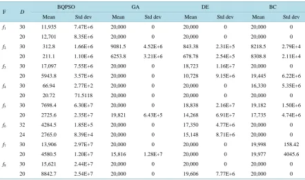
Table 4.Comparison of the mean of the error and the standard deviation of NFE of the four algorithms.

F D BQPSO GA DE BC

Mean Std dev Mean Std dev Mean Std dev Mean Std dev

f1 30 11,935 7.47E+6 20,000 0 20,000 0 20,000 0

20 12,701 8.35E+6 20,000 0 20,000 0 20,000 0

f2 30 312.8 1.66E+6 9081.5 4.52E+6 843.38 2.31E+5 8218.5 2.79E+4

20 211.1 1.10E+6 6253.8 3.21E+6 678.78 2.54E+5 8308.8 2.11E+4 f3 30 17,097 7.55E+6 20,000 0 18,723 1.16E+7 20,000 0

20 5943.8 3.57E+6 20,000 0 10,728 9.15E+6 19,445 6.22E+6 f4 30 66.94 2.77E+2 20,000 0 20,000 0 16,330 5.35E+6

20 20.72 71.5118 20,000 0 20,000 0 20,000 0

f5 30 7698.4 6.30E+7 20,000 0 18,838 2.16E+7 19,182 1.50E+6

20 2725.6 2.35E+7 19,821 6.43E+5 14,268 6.91E+7 17,735 4.74E+6 f6 32 4284.5 1.85E+5 20,000 0 17,350 4.77E+6 20,000 0

24 2765.0 8.39E+4 20,000 0 15,148 8.71E+6 20,000 0 f7 30 13,906 2.97E+7 20,000 0 20,000 0 19,998 158.42

20 4580.5 1.20E+7 15,816 1.28E+7 20,000 0 19,977 4045.6

f8 30 15,621 2.44E+7 20,000 0 20,000 0 20,000 0

20 8842.7 2.54E+7 20,000 0 19,606 7.77E+6 20,000 0

three algorithms. The DE algorithm performed well on average. It obtained the best results among the three al-gorithms for some benchmark functions, but it did not successfully optimize the functions f2, f4, and f7, because it

got trapped in a local optimum. The BC achieved the best results among the three algorithms for the 30-dimensional functions f2, f4, and f7. The GA achieved the best results among three algorithms for the

20-dimensional functions f2 and f7. The DE achieved the best results among three algorithms for the

20-dimensional function f4. According to the experimental results, the algorithms can be ordered by optimizing

performance from high to low as BQPSO, DE, BC, GA. This demonstrates the superiority of BQPSO.

These results can be easily explained as follows. First, In BQPSO, two parameters θ and ϕ of a qubit can be simultaneously adjusted by means of rotating the current qubit through an angle δ about the rotation axis. This rotation can automatically achieve the best matching of two adjustments. In other words, when the current qubit moves towards the target qubit, the path is the minor arc of the great circle on the Bloch sphere, which is clearly the shortest. Obviously, this rotation with the best matching of two adjustments has a higher optimization ability. Secondly, the three chains structure of the encoding particle also enhances the ergodicity of the solution space. These advantages are absent in the other three algorithms.

5. Conclusion

para-meter changes. Further research will focus on enhancing the computational efficiency of BQPSO without re-ducing the optimization performance.

References

[1] Kennedy, J. and Eberhart, R.C. (1995) Particle Swarms Optimization. Proceedings of IEEE International Conference on Neural Networks, 4, 1942-1948. http://dx.doi.org/10.1109/icnn.1995.488968

[2] Guo, W.Z., Chen, G.L. and Peng, S.J. (2011) Hybrid Particle Swarm Optimization Algorithm for VLSI Circuit Parti-tioning. Journal of Software,22, 833-842. http://dx.doi.org/10.3724/SP.J.1001.2011.03980

[3] Hamid, M., Saeed, J., Seyed, M., et al. (2013) Dynamic Clustering Using Combinatorial Particle Swarm Optimization.

Applied Intelligence, 38, 289-314. http://dx.doi.org/10.1007/s10489-012-0373-9

[4] Lin, S.W., Ying, K.C. and Chen, S.C. (2008) Particle Swarm Optimization for Parameter Determination and Feature Slection of Support Vector Machines. Expert Systems with Applications, 35, 1817-1824.

http://dx.doi.org/10.1016/j.eswa.2007.08.088

[5] Yamina, M. and Ben, A. (2012) Psychological Model of Particle Swarm Optimization Based Multiple Emotions. Ap-plied Intelligence, 36, 649-663. http://dx.doi.org/10.1007/s10489-011-0282-3

[6] Cai, X.J., Cui, Z.H. and Zeng, J.C. (2008) Dispersed Particle Swarm Optimization. Information Processing Letters,

105, 231-235. http://dx.doi.org/10.1016/j.ipl.2007.09.001

[7] Bergh, F. and Engelbrecht, A.P. (2005) A Study of Particle Swarm Optimization Particle Trajectories. Information Science, 176, 937-971.

[8] Chatterjee, A. and Siarry, P. (2007) Nonlinear Inertia Weight Variation for Dynamic Adaptation in Particle Swarm Op-timization. Computers & Operations Research, 33, 859-871. http://dx.doi.org/10.1016/j.cor.2004.08.012

[9] Lu, Z.S. and Hou, Z.R. (2004) Particle Swarm Optimization with Adaptive Mutation. Acta Electronica Sinica, 32, 416-420.

[10] Liu, Y., Qin, Z. and Shi, Z.W. (2007) Center Particle Swarm Optimization. Neurocomputing, 70, 672-679. http://dx.doi.org/10.1016/j.neucom.2006.10.002

[11] Liu, B., Wang, L. and Jin, Y.H. (2005) Improved Particle Swarm Optimization Combined with Chaos. Chaos Solitons & Fractals, 25, 1261-1271. http://dx.doi.org/10.1016/j.chaos.2004.11.095

[12] Luo, Q. and Yi, D.Y. (2008) A Co-Evolving Framework for Robust Particle Swarm Optimization. Applied Mathemat-ics and Computation, 199, 611-622. http://dx.doi.org/10.1016/j.amc.2007.10.017

[13] Zhang, Y.J. and Shao, S.F. (2011) Cloud Mutation Particle Swarm Optimization Algorithm Based on Cloud Model.

Pattern Recognition & Artificial Intelligence, 24, 90-95.

[14] Zhu, H.M. and Wu, Y.P. (2010) A PSO Algorithm with High Speed Convergence. Control and Decision, 25, 20-24. [15] Wang, K. and Zheng, Y.J. (2012) A New Particle Swarm Optimization Algorithm for Fuzzy Optimization of Armored

Vehicle Scheme Design. Applied Intelligence, 37, 520-526. http://dx.doi.org/10.1007/s10489-012-0345-0

[16] Salman, A.K. and Andries, P.E. (2012) A Fuzzy Particle Swarm Optimization Algorithm for Computer Communica-tion Network Topology Design. Applied Intelligence, 36, 161-177. http://dx.doi.org/10.1007/s10489-010-0251-2 [17] Mohammad, S.N., Mohammad, R.A. and Maziar, P. (2012) LADPSO: Using Fuzzy Logic to Conduct PSO Algorithm.

Applied Intelligence, 37, 290-304. http://dx.doi.org/10.1007/s10489-011-0328-6

[18] Zheng, Y.J. and Chen, S.Y. (2013) Cooperative Particle Swarm Optimization for Multi-Objective Transportation Plan-ning. Applied Intelligence, 39, 202-216. http://dx.doi.org/10.1007/s10489-012-0405-5

[19] Jose, G.N. and Enrique, A. (2012) Parallel Multi-Swarm Optimizer for Gene Selection in DNA Microarrays. Applied Intelligence, 37, 255-266. http://dx.doi.org/10.1007/s10489-011-0325-9

[20] Sun, J., Feng, B. and Xu, W.B. (2004) Particle Swam Optimization with Particles Having Quantum Behavior. Pro-ceedings of IEEE Conference on Evolutionary Computation, 1, 325-331.

[21] Sun, J., Feng, B. and Xu, W.B. (2004) A Global Search Strategy of Quantum-Behaved Particle Swarm Optimization.

Proceedings of IEEE Conference on Cybernetics and Intelligent Systems, 1, 111-116.

[22] Sun, J., Xu, W.B. and Feng, B. (2005) Adaptive Parameter Control for Quantum-Behaved Particle Swarm Optimiza-tion on Individual Level. Proceedings of IEEE Conference on Cybernetics and Intelligent Systems, 4, 3049-3054. [23] Said, M.M. and Ahmed, A.K. (2005) Investigation of the Quantum Particle Swarm Optimization Technique for

Elec-tromagnetic Applications. Proceedings of IEEE Antennas and Propagation Society International Symposium, Wash-ington DC, 3-8 July 2005, 45-48.

versity. Proceedings of International Conference on Computational Science, University of Reading, 28-31 May 2006, 847-854.

[25] Xia, M.L., Sun, J. and Xu, W.B. (2008) An Improved Quantum-Behaved Particle Swarm Optimization Algorithm with Weighted Mean Best Position. Applied Mathematics and Computation, 205, 751-759.

http://dx.doi.org/10.1016/j.amc.2008.05.135

[26] Fang, W., Sun, J., Xie, Z.P. and Xu, W.B. (2010) Convergence Analysis of Quantum-Behaved Particle Swarm Optimi- zation Algorithm and Study on Its Control Parameter. Acta Physica Sinica, 59, 3686-3693.

[27] Said, M.M. and Ahmed, A.K. (2006) Quantum Particle Swarm Optimization for Electromagnetic. IEEE Transactions on Antennas and Propagation, 54, 2765-2775.

[28] Gao, W.F., Liu, S.Y. and Huang, L.L. (2012) A Global Best Artificial Bee Colony Algorithm for Global Optimization.

Journal of Computational and Applied Mathematics, 236, 2741-2753. http://dx.doi.org/10.1016/j.cam.2012.01.013 [29] Adam, P.P., Jaroslaw, J. and Napiorkowski, A.K. (2012) Differential Evolution Algorithm with Separated Groups for

Multi-Dimensional Optimization Problems. European Journal of Operational Research, 216, 33-46. http://dx.doi.org/10.1016/j.ejor.2011.07.038

[30] Liu, G., Li, Y.X., Nie, X. and Zheng, H. (2012) A Novel Clustering-Based Differential Evolution with 2 Multi-Parent Crossovers for Global Optimization. Applied Soft Computing, 12, 663-681.

http://dx.doi.org/10.1016/j.asoc.2011.09.020

[31] Suganthan, P.N., Hansen, N. and Liang, J.J. (2005) Problem Definitions and Evaluation Criteria for the CEC2005 Spe-cial Session on Real Parameter Optimization. http://www.ntu.edu.sg/home/EPNSugan