The Large Scale Instability in Rotating Fluid with Small Scale Force

(1)

http://dx.doi.org/10.4236/ojfd.2015.52015

The Large Scale Instability in Rotating Fluid

with Small Scale Force

Michael Kopp

1

_{, Anatoly Tur}

2

_{, Vladimir Yanovsky}

1

1_{National Academy of Science Ukraine, Institute for Single Crystals, Kharkiv University, Kharkov, Ukraine} 2_{Institut de Recherche en Astrophysique et Planétologie, CNRS, Université de Toulouse [UPS], Toulouse, France}

Email: [email protected]

This work is licensed under the Creative Commons Attribution International License (CC BY).

http://creativecommons.org/licenses/by/4.0/

Abstract

In this paper, we find a new large scale instability in rotating flow forced turbulence. The turbu-lence is generated by a small scale external force at low Reynolds number. The theory is built on the rigorous asymptotic method of multi-scale development. The nonlinear equations for the in-stability are obtained at the third order of the perturbation theory. In this article, we explain the nonlinear stage of the instability and the generation vortex kinks.

Keywords

Large Scale Vortex Instability, Coriolis Force, Multi-Scale Development, Small Scale Turbulence, Vortex Kinks

1. Introduction

(2)

[image:2.595.205.423.195.415.2]

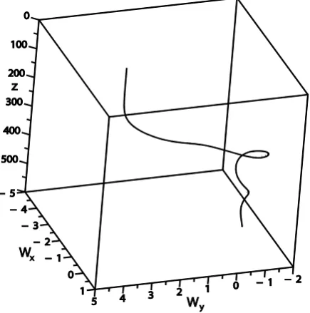
with internal helical structure appear as a result of the development of this instability in rotating fluid. We can consider that external small scale force substitutes the action of small scale turbulence. It is supposed that exter-nal force is in plane (X, Y), which is perpendicular to the rotation axis, for example, axis Z is directed along the vector of angular velocity of rotation Ω. Helical 2D field of velocity Wx, Wy turns around axis Z, when Z changes in the kink which links the hyperbolic point and the stable focus (Figure 1). Moreover, this field does some turns in the kink, which links instable and stable focuses (Figure 2). The found instability belongs to the class of instabilities called hydrodynamic α-effect. For these instabilities, the positive feedback between velocity com-ponents of Wx, Wy is typical.

Figure 1. The kink which connects the hyperbolic point with stable knot with D = 1, C1 = 0.04, C2 = 0.04. When ap-proaching the stable knot one can see rotations of velocity field.

[image:2.595.203.423.471.682.2]

(3)

0,

TWx Wx y Wy

z

α ∂

∂ − ∆ − =

∂

0,

TWy Wy x Wx

z

α ∂

∂ − ∆ + =

∂

and leads to the instability. The α-effect is taking its origins from magnetic hydrodynamics, where it engenders the increase of large scale magnetic fields (see for example [16]). It was generalized later for ordinary hydrody-namics. For the time being some examples of hydrodynamics α-effect [8]-[14] are already known. From this point of view, in this work we found a new example of α-effect. The theory of this instability is developed ri-gourously using the method of asymptotic multi-scale development, similar to what was done by Frisch, She and Sulem for the theory of the AKA effect [13]. This method allows finding the equations for large scale perturba-tions as secular equaperturba-tions of asymptotical theory in order to calculate the Reynolds stress tensor and to find the instability. The small parameter of asymptotical development is the Reynolds number R, R1. Our paper is organised as follows: in Section 2 we formulate the problem and the main equations in rotating system of coor-dinates; in Section 3 we examine the principal scheme of the multi-scale development and we give the secular eq-uations. In Section 4 we calculate the velocity field of zero approximation. In Section 5 we describe the calcula-tions of the Reynolds stress and find the large scale instability. In Section 6 we discuss the saturation of the in-stability and find non linear stationary vortex structures. The results obtained are discussed in the conclusions given in Section 7.

2. The Main Equations and Formulation of the Problem

Let us examine the equations of motion for non-compressible rotating fluid with external force F₀ in rotating coordinates system:

( )

0

1

2 P ,

t ρ ν

∂

+ ∇ + × = − ∇ + ∆ +

∂

V

V V Ω V V F (1)

0.

divV = (2) The external force F0 is divergence-free. Here Ω-angular velocity of fluid rotation, ν -viscosity, ρ0-con- stant fluid density. Let us design characteristic amplitude of force f0, and its characteristic space and time scale

0

λ and t₀ respectively.

Then ₀ ₀ ₀ 0 0

,t

f

t

λ

 

= _ _

 

x

F F . We will design the characteristic amplitude of velocity, generated by external

force as v₀. We choose the dimensionless variables

(

t x V, ,

)

: 0 0

0 0 0 0 0 0

2 2

0 0 0 0 0

0 0 0 2 0

0 0

, , , , ,

, , , .

t P

t v f P

v v f

t P f v

λ ρ

λ ν ν λ

ν λ λ ν

→ → → → →

= = = =

F

x V

x V F

Then, in dimensionless variables the Equation (1) takes forme:

(

)

0,

R P

t

∂ ₊ _⋅∇ _{+ × = −∇ + ∆ +}

∂

V

V V D V V F (3)

0 0v

R λ

ν

= , D = Ta where R and

2 4 0 2 4

Ta λ

ν

Ω

(4)

say, they are large scale. From a formal point of view, these terms are secular, i.e., they create the conditions for the solvability of a large scale asymptotic development. So the purpose of this paper is to find and study the solvability equations, i.e., the equations for large scale perturbations. Let us denote the small scale variables by

(

)

0 0, 0

x = x t , and the large scale ones by X =

(

X,T

)

. The small scale partial derivative operation

0 i x ∂ ∂ , t0

∂

∂ , and the large scale ones

∂ ∂X , T

∂

∂ are written, respectively, as ∂i, ∂t, ∇i and ∂T. To con-struct a multi-scale asymptotic development we follow the method which is proposed in [16].

3. The Multi-Scale Asymptotic Development

Let us search for the solution to Equations (2) and (3) in the following form:

( )

2 3

1 0 0 1 2 3

1

,t X x R R R ,

R −

= + + + + +

V x W v v v v  (4)

( )

2 3

1 0 0 1 2 3

1

, ,

T t T X T x RT R T R T R −

= + + + + +

x  (5)

( )

₍

( )

₎

2 3

3 2 1 0 0 1 1 2 3

3 2

1 1 1

, .

P t P X P X P X P x R P P X R P R P

R

R − R − −

= + + + + + + + +

x  (6)

Let us introduce the following equalities: X =R2x0 and 4

0

T =R t which lead to the expression for the space and time derivatives:

2

,

i i

i R

x

∂ _{= ∂ + ∇}

∂ (7)

4

,

t R T t

∂ _{= ∂ + ∂}

∂ (8) 2

2 4

2 .

jj j j jj

j j R R

x x

∂

= ∂ + ∂ ∇ + ∂

∂ ∂ (9)

Using indicial notation, the system of equation can be written as

(

)

(

)(

)

(

) (

)

4 2

2 2 4

0

2 ,

i i j j k

t T j j ijk

i i

j j jj j j jj

R V R R V V D V R P R R V F

ε

∂ + ∂ + ∂ + ∇ +

= ∂ + ∇ + ∂ + ∂ ∇ + ∇ + (10)

( )

,

z i

tT jjT V R j V T

∂ − ∂ = − − ∂ (11)

(

2

)

0.

i i R i V

∂ + ∇ = (12) Substituting these expressions into the initial Equations (2) and (3) and then gathering together the terms of the same order, we obtain the equations of the multi-scale asymptotic development and write down the obtained equations up to order R3 inclusive. In the order R−3 there is only the equation

( )

3 0 3 3 .

iP− P− P− X

∂ = ⇒ = (13) In order R−2 we have the equation

( )

2 0 2 2 .

iP− P− P− X

∂ = ⇒ = (14)

In order R−1 we get a system of equations:

(

)

1 1 1 1 3 1 1,

i i j k i j

tW− jjW− D

ε

ijkW− iP− iP− jW W− −

∂ − ∂ + = − ∂ + ∇ − ∂ (15)

1 0. i iW−

∂ =

The system of Equations (17) and (18) gives the secular terms

3 1,

j k

iP− D

ε

ijkW−

(5)

which corresponds to a geostrophic equilibrum equation. In zero order R0, we have the following system of equations:

(

)

(

)

0 0 1 0 0 1 0 0 2 0,

i i i j i j j k i

tv jjv j W v− v W− Dεijkv iP iP− F

∂ − ∂ + ∂ + + = − ∂ + ∇ + (17)

0 0. i iv

∂ =

These equations give one secular equation:

2 0 2 Const.

P− P−

∇ = ⇒ = (18) Let us consider the equations of the first approximation R:

(

)

(

)

(

)

1 1 1 1 1 1 1 0 0 1 1 1 1 ,

i i j k i j i j i j i j

tv jjv Dεijkv j W v− v W− v v j W W− − iP iP−

∂ − ∂ + + ∂ + + = −∇ − ∂ + ∇ (19)

1 1 0.

i i

iV iW−

∂ + ∇ = (20) From this system of equations there follows the secular equations:

1 0, i iW−

∇ = (21)

(

1 1

)

1.

i j

j W W− − iP−

∇ = −∇ (22) The secular Equations (27) and (29) are satisfied by choosing the following geometry for the velocity field (Beltrami field):

( )

(

1 , 1 , 0 ;

)

x y

W− Z W− Z =

W (23)

1 0 1 Const.

P− P−

∇ = ⇒ =

In the second order R2, we obtain the equations

(

)

(

)

(

)

2 2 0 1 2 2 1 0 1 1 0 2

1 0 0 1 2 0

2

,

i i i i j i j i j i j j k

t jj j j j ijk

i j i j

j i i

v v v W v v W v v v v D v

W v v W P P

ε

− −

∂ − ∂ − ∂ ∇ + ∂ + + + +

= −∇ + − ∂ + ∇ (24)

2 0 0.

iv iv

∂ + ∇ = (25) It is easy to see that there are no secular terms in this order.

Let us come now to the most important order R3. In this order we obtain the equations

(

)

(

)

(

)

(

)

3 1 3 1 1 1 1 1 1 0 0

1 3 3 1 0 2 2 0 1 1 3 3 1

2

,

i i i i i i j i j i j

t T jj j j jj j

i j i j i j i j i j j k

j ijk i i

v W v v W W v v W v v

W v v W v v v v v v D ε v P P

− − − −

− −

∂ + ∂ − ∂ + ∂ ∇ + ∇ + ∇ + +

+∂ + + + + + = − ∂ + ∇ (26)

3 1 0.

iv iv

∂ + ∇ =

From this we get the main secular equation:

( )

1 1 0 0 1.

i i k i

TW− W− k v v iP

∂ − ∆ + ∇ = −∇ (27)

There is also an equation to find the pressure P−₃:

3 1.

j k

iP− D

ε

ijkW−

−∇ = (28)

4. The Velocity Field in Zero Approximation

It is clear that the most important is Equation (36). In order to obtain these equations in closed form, we need to calculate the Reynolds stresses ∇_k

( )

v v_{0 0}k i . First of all we have to calculate the fields of zero approximation v₀k. From the asymptotic development in zero order we have

0 0 1 0 0 0 0.

i i k i j k i

tv jjv W− kv D

ε

ijkv iP F

(6)

Let us introduce the operator Dˆ₀:

0

ˆ k _.

t jj k

D ≡ ∂ − ∂ +W ∂ (30) Using Dˆ₀, were write Equations (29):

0 0 0 0 0

ˆ i j k i_.

ijk i

D v +D

ε

v = −∂P +F (31) Pressure P₀ can be found from condition divV =0.

[

]

0

0 2 .

i iv

P = ×

∂

D ∂

(32)

Let us introduce designations for operatores:

[

]

2

ˆ i

ij j

P = ∂ ×

∂

D ∂

(33)

and for velocities: v₀x =u₀, v₀y=v₀, v₀z=w₀. Then excluding pressure from (31), we obtain the system of equations to find the velocity field of zero approximation:

 

(

)

(



)

(



)



(

)

(

 

)

(



)



(

)

(



)

(

 

)

0 0 0 0 0

, , .

x

xx yx z zx y

y

xy z yy zy x

z

xz y yz x zz

D P u P D v P D w F P D u D P v P D w F P D u P D v D P w F

+ + − + + =

+ + + + − =

− + + + + =

(34)

For simplicity, we choose the systeme of coordinates so that the axis Z coincides with the direction of angular velocity of rotation Ω. Then Dx=0, Dy=0, Dz=D In order to solve this system of equations we have to set the force in the explicit form.Let us choose now the external force in the rotating system of coordinates in the following form:

(

)

(

)

(

)

0 0 0 2 1 1 1 0 2 2 0

1 0 2 0

0, Cos Cos ; , ,

1, 0,1 , 0,1,1 .

z

F f t t

k k

ϕ ϕ ϕ ω ϕ ω

⊥

= = + = − = −

= =

F i j k x k x

k k

It is obvious that divergence of this force us equal to zero. Thus, external force is given in plane (x, y), ortho-gonal to rotation axis.

The solution for equations system (34) can be found easily in accordance with Cramer’s Rule: 3

1 2

0 , 0 , 0 .

u =∆ v =∆ w =∆

∆ ∆ ∆ (35) Here Δ is the determinant of the system (34):

   

0

,

xx yx zx

xy yy zy

xz yz zz

D P P D P

P D D P P

P P D P

+ −

∆ = + +

+

(36)

 

  

0

1 0 0

0

,

0

x

yx zx

y

yy zy

yz zz

F P D P

F D P P

P D P

−

∆ = +

+

(37)

  

 

  

0 0

2 0

0

,

0

x

xx zx

y

xy zy

xz zz

D P F P

P D F P

P D P

+

∆ = +

+

(7)

  

 

0 0

3 0 0 .

0 x xx yx y xy yy xz yz

D P P D F

P D D P F

P P

+ −

∆ = + + (39)

After writing down the determinants in the explicit form, we obtain:

 

(

)

(

 

)

( )



( )



( )



(



)

(

 

)

0 0 0 0

0 0

1

,

x

yy zz yz zy

y

zx yz yx zz

u D P D P P P F

P P P D D P F

  = _ + + − _ ∆   + _ − − + _ ∆ (40) 

( )



(



)

(

 

)

 

(

)

(

 

)

( )



( )



0 0 0

1

,

x

xz zy xy zz

y

xx zz xz zx

v P P P D D P F

D P D P P P F

  = − + +   ∆   + _ + + − _ ∆ (41) 

(

)

( )



( )



(

 

)



( )

(



)

(

 

)

( )



0 0 0

0 0

1

.

x

xy yz xz yy

y

xz yx xx yz

w P D P P D P F

P P D D P P F

  = _ + − + _ ∆   + _ − − + _ ∆ (42)  

(

)

(

 

)

(

 

)

( )



( )

 

(

)

(



)

(

 

)

( )



( )

 

( )

(



)

( )



(

 

)

( )



0 0 0

0

0 .

xx yy zz yz zy

yx xy zz xz zy

zx xy yz yy xz

D P D P D P P P

P D P D D P P P

P P D P D P P

  ∆ = + _ + + − _   − − _ + + − _   + _ + − + _ (43)

In order to calculate the expressions (40)-(43) we present the external force in complex form:

(

2 2

)

(

1 1

)

0 0

0 e e , 0 e e .

2 2

i i i i

x f y f

F = ϕ + −ϕ F = ϕ + −ϕ (44) Then all operators in formulae (40)-(42) act from the left on their eigenfunctions. In particular:

 

₍

₎

 

₍

₎

(

)

(

)

2 2 1 1

0 0 2 0 0 0 1 0

2 0 1 0

e e , , e e , ,

e e , , e e , .

i i i i

D ϕ ϕ D D ϕ ϕ D

ϕ ϕ ϕ ϕ

ω ω ω ω = − = − ∆ = ∆ − ∆ = ∆ − k k k k (45)

To simplify the formulae, let us choose k₀ =1, ω =₀ 1. We will designate



₍

₎

(

)



₍

₎

₍

₎

0 2, 0 2 y 1 y, 0 1, 0 2 x 1 x.

D k −ω = +i w − =A D k −ω = +i w − =A (46) Before doing further calculations, we have to note that some components of tensors P kˆ_ij

( )

₁ and P kˆ_ij

( )

₂ vanish. Let us write the non-zero components only:

( )

1

( )

2

( )

2

( )

1

1 1 1 1

ˆ _, ˆ _, ˆ _, ˆ _.

2 2 2 2

yx xz xy yz

P k = D P k = − D P k = − D P k = D (47)

Taking into account the formulae (45)-(47), we can find the determinant:

( )

3 2

( )

3 2

1 2

1 1

, .

2 2

x x y y

A D A A D A

∆ k = + ∆ k = + (48)

In a similar way we find velocity field of zero approximation:

2 1

0 0 0

2 2 2 2

e e . ., 1 1 2 4 2 2 i i y y x A D

u f f C C

A D A D

ϕ ϕ

= + +

+ +

(8)

2 1

0 0 0

2 2 2 2

e e . ., 1 1 4 2 2 2 i i x y x A D

v f f C C

A D A D

ϕ ϕ

= − + +

+ +

(50)

2 1

0 0 0

2 2 2 2

e e . .. 1 1 4 4 2 2 i i y x D D

w f f C C

A D A D

ϕ ϕ

= − +

+ +

(51)

5. Reynolds Stress and Large Scale Instability

To close the Equations (27) we have to calculate the Reynolds stresses w u_{0 0} and w v_{0 0}. These terms are easily calculated with help of formulae (49)-(51). As a result we obtain:

2 2 2

0 0

0 0 2 2

2 2 2 2

2 2 2

0 0

0 0 2 2

2 2 2 2

,

2 1 8 1

2 2

.

8 ₁ 2 ₁

2 2

y x

f D f D

w u

A D A D

f D f D

w v

A D A D

= −

+ +

= − −

+ +

(52)

Now Equations (27) are closed and take form:

0 0

0 0 0,

0.

T x x

T y y

W W w u z W W w v

z ∂ ∂ − ∆ + = ∂ ∂ ∂ − ∆ − = ∂ (53)

We calculate the modules and write the Reynolds stresses (52) in the explicit form:

(

)

(

)

(

)

(

)

(

)

(

)

(

)

(

)

2 2 2

0 0

0 0 2 2

2 2 2 2 2 2

2 2 2

0 0

0 0 2 2

2 2 2 2 2 2

,

2 ₁ 8 ₁

16 1 4 1 16 1 4 1

2 2

8 1 2 1

16 1 4 1 16 1 4 1

2

.

2

y y x x

f D f D

w u

w D w w D w

f D f D

w v

w D w w D w

= −     − +_ + − − _ − +_ + − − _     = − −     − +_ + − − _ − +_ + − − _     (54)

With small Wx, Wy Reynolds stresses (52) can be expanded in a series in the small parameters Wx, Wy. Taking into account the formula:

(

)

(

)

2

,

2 ₂ 2

2 2 2 , 32 10 1 Const.

1 ₆ ₆₄

2 x y x y D w D A D − = − +  ₊ ₊  + __ __ 

We obtain the linearized Equations (53):

(

)

(

)

2 2 2

2

0 0

2

2 2 2

2 0 0 2 2 2 2 2 0, 2 8 0. 8 2 32 10 . 6 64

x x y x

y y y x

f D f D

W W W W

T z z z

f D f D

W W W W

T z z z

D D α α α α α ∂ ₋ ∂ ₋ ∂ ₊ ∂ ₌ ∂ ∂ ∂ ∂ ∂ ₋ ∂ ₊ ∂ ₊ ∂ ₌ ∂ ∂ ∂ ∂ − =  ₊ ₊      (55)

(9)

(

)

, exp .

x y

W W ∼

γ

T+ikZ (56) We substitute (56) in Equation (55) and obtain the dispersion equation:

2 2 2

2

0 0 _.

8 2

f D f D ikα kα k

γ = − ± − (57)

The dispersion Equation (57) shows that equation system (55) has instable oscillatory solutions with oscilla-tory frequency 2 2 0 8 f D kα

ω= and instability growth rate

2 2 0 . 2 f D

k

α

k

γ

= − The instability is large scale

be-cause the instable term dominates over dissipation on large scales: 2 0 . 2 f D k

α

 The maximum growth rate of

instability is equal to

2 4 2 0

max ,

16

f D

α

γ = and is achieved on the wave vector

2 0

max .

4

f D

k =

α

As a result of the development of instability the large scale helical circular polarized vortices of Beltrami type are generated in the system.

6. Saturation of Instability and Nonlinear Vortex Structures

It is clear that with increasing of amplitude nonlinear terms decrease and instability becomes saturated. Conse-quently stationary nonlinear vortex structures are formed. To find these structures let us choose for Equations

(54) 0

T ∂ ₌

∂ and integrate equations one time over Z. We obtain the system of equations:

0 0 1

0 0 2 d d d . d , x y

W w u C Z

ZW w v C

= +

(58)

From Equations (58) follows:

0 0 1

0 0 2 , d

d

x y

w u C w w v C w + +

= (59)

After integrating the system of Equations (59) we obtain:

0 0d x 2 x 0 0d y 1 y. w v w +C w = w u w +Cw

∫

(60)

Integrals in expression (60) are calculated in elementary functions (see [17]), which give the expression for first integral of motion J of Equations (59):

(

)

(

)

(

)

(

) (

)

(

) (

)

(

)

(

)

(

)

₍

₎

₍

₎

(

)

(

) (

)

(

) (

)

2 2 2

2 5 2 2 ₂

2 2 2 2 2 2 2 2 2 2 2 2 2 2

5 2 2 2 ₂

1

1 1 2 4

2 ln

1

8 1 2 8 ₁ ₁ ₂ ₄

4 1 16 1 ₂

2

1

1 4

2 arctg

4 1 8

8 8 1

4 1 16 1

2 1

1 1 2 4

2 ln

1

2 8 ₁ ₁ ₂ ₄ 8 8

2 x x x x x y y x y x x x y y y y

w w D D

w

D D

J

D _w _w _D _D

D w w

w D _w

D D

w D

D w w

w w D D

D D

D _w _w _D _D D

− + − + + = + +  ₊ ₋ ₋  ₊ ₋ ₋ ₋ ₋ _{+ +}     − − − + − − +  ₊ ₋ ₋  ₊ ₋     − + − + + + + + ₋ ₋ ₋ _{+ +}

(

+

)

(

)

(

)

2 2 1 2 2 1 1 4 2 arctg . 4 1 y y x y w D

C w C w w

− − −

+ +

−

(10)

[image:10.595.221.406.82.251.2]

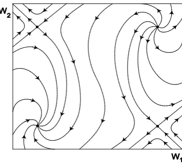
Figure 3. Phase portrait of the dynamical system (58), with D = 1, C1 = −0.03, C2 = 0.03. One can see two hyperbolic singular points and stable and instable knots.

the stable knot and Figure 2, where the solution connects instable and stable focuses. All these solutions cor-respond to the large scale localized vortex structures of kink type with rotation, generated by the instability which has been found in this work.

7. Conclusions and Discussion of the Results

In this work we find the new large scale instability in rotating fluid. It is supposed that the small scale vortex external force in rotating coordinates system acts on fluid which maintains the small velocity field fluctuations (small scale turbulence with small Reynolds number R, R1). For the real applications this Reynolds number should be calculated with help of the turbulent viscosity. The asymptotic development of motion equations by small Reynolds number allows obtaining motion equations for the large scale. These equations are of the hy-drodynamic α-effect type, in which velocity components Wx, Wy are connected by the positive feedback. This may result in the appearance of the large scale vortex instability. The large scale vortices of Beltrami type are formed due to this instability in rotating fluid with small scale exterior force. With further increase of amplitude, the instability stabilizes and passes to stationary mode. In this mode the nonlinear stationary vortex structures form. Different vortex kinks belong to the most interesting structures. These kinks link stationary points of dy-namical system (58). Kinks which link the hyperbolic point with the stable knot rotate around the stable knot as shown on Figure 1. In the kink which links instable and stable focuses, vector field turns around two singular points, see Figure 2.

Let us note that unlike previous works about hydrodynamic α-effect in rotating fluid, the use of the asymptot-ic development allows constructing naturally the nonlinear theory and studying the stationary nonlinear vortex kinks.

References

[1] Grinspen, H.P. (1990) The Theory of Rotating Fluids. Breukelen Press, Brookline.

[2] Roberts, P.H. and Soward, A.M. (1978) Rotating Fluids in Geophysics. Academic Press, London.

[3] Clarke, C. and Carswell, B. (2007) Principles of Astrophysical Fluid Dynamics. Cambridge University Press, Cam-bridge. http://dx.doi.org/10.1017/CBO9780511813450

[4] Vallis, G.K. (2010) Atmospheric and Oceanic Fluid Dynamics. Cambridge University Press, Cambridge.

[5] Abramowicz, M.A., Lanza, A., Spigel, E.A. and Szuszkiewicz, E. (1992)Vortices on Accretion Disks. Nature, 356, 41-43. http://dx.doi.org/10.1038/356041a0

[6] Brandt, P.N., Scharmer, G.B., Ferguson, S., Shine, R.A., Tarbell, T.D. and Title, A.M. (1988)Vortex Flow in the Solar Photosphere. Nature, 335, 238. http://dx.doi.org/10.1038/335238a0

(11)

http://dx.doi.org/10.1063/1.881375

[8] Moiseev, S.S., Sagdeev, R.Z., Tur, A.V., Khomenko, G.A. and Yanovsky, V.V. (1983) A Theory of Large-Scale Structure Origination in Hydrodynamic Turbulence. Soviet Physics—JETP, 58, 1149.

[9] Moiseev, S.S., Rutkevich, P.B., Tur, A.V. and Yanovsky, V.V. (1988) Vortex Dynamos in a Helical Turbulent Con-vection. Soviet Physics—JETP, 67, 294.

[10] Lupyan, E.A., Mazurov, A.A., Rutkevich, P.B. and Tur, A.V. (1992) Generation of Large-Scale Vortices through the Action of Spiral Turbulence of a Convective Nature. Soviet Physics—JETP, 75, 833.

[11] Khomenko, G.A., Moiseev, S.S. and Tur, A.V. (1991) The Hydrodynamic Alpha-Effect in a Compressible Fluid.

Journal of Fluid Mechanics, 225, 355. http://dx.doi.org/10.1017/S0022112091002082

[12] Levina, G.V., Moiseev, S.S. and Rutkevich, P.B. (2000) Hydrodynamic Alpha-Effect in a Convective System. Ad-vances in Fluid Mechanics, 25, 111.

[13] Frisch, U., She, Z.S. and Sulem, P.L. (1987) Large-Scale Flow Driven by the Anisotropic Kinetic Alpha Effect. Physi-ca D, 28, 382. http://dx.doi.org/10.1016/0167-2789(87)90026-1

[14] Tur, A.V. and Yanovsky, V.V. (2013) Non Linear Vortex Structures in Stratified Fluid Driven by Small-Scale Helical Force. Open Journal of Fluid Dynamics, 3, 64. http://dx.doi.org/10.4236/ojfd.2013.32009

[15] Kitchatinov, L.L., Rudiger, G. and Khomenko, G. (1994) Large-Scale Vortices in Rotating Stratified Disks. Astronomy & Astrophysics, 287, 320.

[16] Moffat, H.K. (1978) Magnetic Field Generation in Electrically Conducting Fluids. Cambridge University Press, Cam-bridge.