Exchange rate in transition

Munich Personal RePEc Archive

Exchange rate in transition

Kocenda, Evzen

Charles University, CERGE

1998

Online at https://mpra.ub.uni-muenchen.de/32030/

Exchange Rate in Transition

Evžen Kocenda

CERGE, Charles University

Published by:

CERGE

Charles University Politických veznu 7 111 21 Praha 1

© Evžen Kocenda, 1998

Reviewed by: Jan Hanousek

Preface

In this book several econometric techniques are used to perform quantitative research of the exchange rate in transition. This is an empirical work based on related economic theory. While the stress is put on the exchange rate of the Czech koruna, the subject is analyzed from a broader perspective of other transition countries as well. I have used parts of the original text in my class Econometrics IV (Applied Time Series) that I teach at CERGE of Charles University.

Contents

1 Introduction 1

2 Conditional variance analysis of the exchange rate 6

2.1 Exchange rate environment 6

2.2 Data and the currency basket 7

2.3 Process underlying exchange rate movement 11

2.4 Conditional variance 15

2.5 Testing the fit of the model 20

2.6 Empirical summary 25

3 Volatility of exchange rate with change in fluctuation band 27

3.1 Altered band 27

3.2 Data 28

3.3 Leverage effect 29

3.4 Leverage effect empirics in exchange rate 31

3.5 Brief summary 34

4 Intratemporal links among interest and exchange rates 36

4.1 Basic facts 36

4.2 Vector autoregressive analysis of lead-lag relationship 38

4.3 Data 41

4.4 Intratemporal linkages 41

4.5 Comments and implications 49

5 Convergence of exchange rates 51

5.1 Exchange rate and its regime in transition countries 51

5.2 Data and definitions 70

5.3 Methodology of convergence 72

5.4 Empirical results of convergence analysis 77

5.5 Concluding observations 83

1

Introduction

At this point, nearly a decade into transition, the Czech Republic has completed the early stages of the process. The country has launched various privatization programs and has adopted an extensive range of measures to implement monetary and fiscal policies that would suit the needs of the overall transformation. Aside from private investors, numerous international organizations have become involved to aid the process. Naturally, the country recorded both achievements and failures. Any country in transition must undergo a stage of macroeconomic stabilization, which is inevitably accompanied by large shocks to macroeconomic fundamentals. The nature and magnitude of these disruptions affect the progress of economic development. Research into the success of the stabilization programs in transition economies is especially important for policymakers. Owing to the relative openness and the close economic relations among transition economies in Central and Eastern Europe and between these countries and the European Union, the exchange rate and the exchange rate regime play an important role in economic development.

The stability of the exchange rate and a type of its regime are important elements in the overall monetary policy of each country. The significance of the matter is even more accentuated in the case of transition economies because international lending institutions like the International Monetary Fund, the World Bank, and the European Bank for Reconstruction and Development provide credit subject to macroeconomic stability and a stable exchange rate. This is true no matter what kind of regime is adopted.

countries from the beginning of the transformation until recently. The overall analysis is based on an economic theory and applies both classical and advanced econometric techniques. Thus, the theoretical approach allows the formulation of qualified empirical conclusions.

Chapter 2 concentrates on a conditional variance analysis of the exchange rate of the Czech koruna. Several detailed studies have applied the generalization of the autoregressive conditional heteroskedastic (ARCH) model to assess the changing variances of exchange rates and their distribution. Knowledge of the exchange rate behavior has important implications for the decisions made in an international financial environment. The opening of new emerging markets in Central and Eastern Europe has increased interest in exploring the behavior of the exchange rates of the region. Central and Eastern European economies are undergoing a unique transformation and for these reasons their exchange rate arrangements differ from those in the developed economies.

This chapter examines the behavior of the exchange rate of the Czech koruna when pegged to a currency basket. This is a significant contribution to the field because, so far, no research has applied the ARCH model to such an exchange rate. The exchange rates are described both narratively and from a statistical point of view. A short explanation is provided on how the exchange rate movement is related to the currency basket peg. The peg is supposed to limit the overall instability of the currency, and hence, stabilize the exchange rate. This is conditional on the central bank keeping the index of the currency basket within a narrow band without subjective tampering. If inconsistency occurs, the pegged rates do not fully reflect the underlying processes in free exchange rates and further analysis is futile.

account for heteroskedasticity. Estimates of the models are presented separately for the mean and variance equations along with statistical tests that show comparable as well as differing results from referenced studies. A separate section elaborates on the nonlinearity in exchange rate movement and uses an advanced nonparametric BDS statistic to test the results. The quantitative results are applied to the behavior of exchange rates and central bank policy.

Chapter 3 extends the analysis from the previous chapter and presents a modification of the technique used. This part examines the behavior of the exchange rate of the Czech koruna when pegged to a currency basket under different fluctuation bands. The currency basket peg is supposed to limit the overall instability of the currency. Such limiting means stabilizing the exchange rate and lowering its volatility. Again, this is conditional on the central bank keeping the index of the currency basket within a narrow band. The purpose of the analysis is to show how the volatility of the exchange rate is affected by allowing for a wider fluctuation band.

The GARCH-L(1,1) model with a dummy variable for the volatility response to the koruna’s appreciation in a variance equation is applied in order to model conditional variance in exchange rates. This is done in order to account for the change in the width of the fluctuation band. Estimates of the models are presented for the mean and variance equations. The results show that, contrary to conventional wisdom, the volatility of the various exchange rates decreased after a much wider fluctuation band was introduced to limit movements of the currency basket index.

chapter 4 where we analyze the linkages between interest rates, as well as interest rates and exchange rates, and compare the results of the periods before 1997 with those in the year, when the country experienced financial crisis. The concept of Granger causality within the framework of the bivariate Vector Autoregressive model is used as an econometric tool to test the respective hypotheses.

The relatively stable environment of the fixed exchange rate regime and semi-regulated interest rates provided a soft environment for the evolution of links among key interest rates and the exchange rate. The bonds among interest rates tended to evolve in a weak economic sense. During the turbulent times of the financial crisis, the prevailing links among interest rates tended to gain strength and the money market became more efficient than ever before. The evolution of the linkages also showed that interest rates influenced the exchange rate during the year of crisis. The exchange rate was found to influence only the short-term interest rates.

The broader perspective of exchange rate analysis among Central and Eastern European countries is discussed in chapter 5. Here we address the question of whether the transition countries have achieved exchange rate development that would eventually lead to greater similarities with the countries within the European Union.

2

Conditional variance analysis of the exchange rate

2.1 Exchange rate environment

In 1991, former Czechoslovakia officially started its economic transformation. From this time the role of the exchange rate could no longer be disfigured as in the former centrally planned economy. However, a certain reduction in the relative volatility of exchange rates was desirable in order to promote export, direct foreign investments and generally favorable economic development during the transition to a free market economy. With the absence of fully functioning financial markets, the newly emerged private sector was extremely vulnerable to exchange rate fluctuations. The fixed exchange rate provided a less volatile environment according to policy makers at that time.

The shock of the transition needed to be buffered, and therefore, to introduce a floating exchange rate system would have been premature. A floating exchange rate regime requires that no restrictions on financial capital movement be imposed. This necessitates a strong mature economy with sufficient reserves of convertible currencies. During the early stages of economic reform, the country did not meet these conditions and an eventual bank run could have caused vast damage. The situation resulted in a temporary anchor of the currency basket peg. We will define currency basket and describe its properties in the next section. Further, additional detailed discussion on the role of fixed exchange rates can be found in Svensson (1994).

convertibility of the koruna was implemented on October 1, 1995, and meant that the koruna could be traded for foreign exchange without restrictions by both companies and citizens. However, this step was not paired with any change in the exchange rate regime and the koruna remained pegged to the currency basket. Thus, after this date, the exchange rate of the koruna was still not completely free to float as the currencies of developed economies. We now proceed to statistical description of exchange rates in question as well as of a currency basket.

2.2 Data and the currency basket

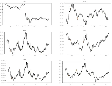
The data consists of daily midpoint exchange rates of the Czech koruna (CZK) to six major currencies during the period from January 2, 1991 to September 30, 1994. The split-up of the former Czechoslovakia on January 1, 1993 generated two separate currencies (Czech koruna and Slovak koruna) which replaced the former Czechoslovak koruna. The entire series is referred to as the Czech koruna because it (CZK) followed the former stable path of the old Czechoslovak koruna. After the monetary separation the Slovak koruna has devaluated considerably. The data was supplied by the Czech National Bank (CNB), Prague. Six major currencies were selected for this study because of their importance in international trade and their inclusion in the currency basket to which the Czech koruna is pegged. The rates of foreign currencies in terms of the Czech koruna are: British Pound (GBP), Austrian Shilling (ATS), Deutsche Mark (DEM), U.S. Dollar (USD), Swiss Franc (CHF), and French Franc (FRF). There are a total of 953 daily observations for each currency.

Table 2.1 Summary statistics of log price changes: rt = log(Rt/Rt-1)*100

Statistics GBP ATS DEM USD CHF FRF

Mean -0.02163 -0.00242 -0.00416 0.00534 -0.00156 -0.00447 Variance 0.23785 0.12908 0.11577 0.22176 0.20454 0.12005 Skewness -1.68703 -0.40586 -0.57688 0.34574 -0.16915 -0.76434

Kurtosis 16.2077 2.35196 3.21914 1.65811 2.57694 6.27226 Maximum 1.99089 1.53259 1.28961 2.45490 2.28472 1.49497 Minimum -4.9373 -1.19121 -1.73237 -1.69109 -2.34774 -2.75034

Figure 2.1 Evolution of Exchange Rates: Nominal Levels

GBP

91 92 93 94

40 42 44 46 48 50 52 54 ATS

91 92 93 94

2.44 2.48 2.52 2.56 2.60 2.64 2.68 2.72 DEM

91 92 93 94

17.00 17.25 17.50 17.75 18.00 18.25 18.50 18.75 19.00 19.25 USD

91 92 93 94

26.6 27.3 28.0 28.7 29.4 30.1 30.8 31.5 CHF

91 92 93 94

18.5 19.0 19.5 20.0 20.5 21.0 21.5 22.0 FRF

91 92 93 94

4.9 5.0 5.1 5.2 5.3 5.4 5.5 5.6 5.7

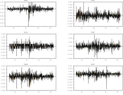
Figure 2.1 shows the evolution of the respective exchange rates over the entire period. The data are not stationary but are a first-order integrated process. The rate of change is calculated by taking the logarithmic difference between two consecutive business days. Figure 2.2 represents the logarithmic first order differences of exchange rates. It serves as a visual test for stationarity and illustrates the periods of volatility.

Figure 2.2 First Logarithmic Differences of Exchange Rates

GBP

91 92 93 94

-0.05 -0.04 -0.03 -0.02 -0.01 0.00 0.01 0.02 ATS

91 92 93 94

-0.020 -0.015 -0.010 -0.005 0.000 0.005 0.010 0.015 0.020 DEM

91 92 93 94

-0.020 -0.015 -0.010 -0.005 0.000 0.005 0.010 0.015 USD

91 92 93 94

-0.020 -0.015 -0.010 -0.005 0.000 0.005 0.010 0.015 0.020 0.025 CHF

91 92 93 94

-0.024 -0.016 -0.008 0.000 0.008 0.016 0.024 FRF

91 92 93 94

-0.030 -0.025 -0.020 -0.015 -0.010 -0.005 0.000 0.005 0.010 0.015

In order to address properly the question of how the exchange rate behaved during the researched period we introduce a short description of the monetary instrument called currency basket. The currency basket was primarily meant to be a nominal anchor that allows, under a prudent policy, to keep a relatively stable nominal exchange rate. Currency is pegged to a currency basket when it is bound to several currencies via

rate arrangement. The CNB introduced the basket system at its current general level at the beginning of 1991 and constructed the basket as a weighted average of nominal exchange rates. The use of weighted average mathematically creates a slight discrepancy by not fully exploiting the importance of the respective currencies, which are represented by their weights. This would be eliminated by using a geometric average instead.

The change in the value of the currency basket is measured by its index

I(t,w), which the CNB defines as

( )

_∑

[

( ) ( )

]

=

= N

j

j j

j R t R

w w

t I

1

0 /

, (2.1)

where wjis a weight (

∑

time t, and Rj(0) is the domestic exchange rate at time 0, i.e. the base exchange rate. Both rates are at nominal levels. In order to peg the home currency to a currency basket, the index must be fixed. In this case it means that the index is set to be equal to one (I(t,w) = 1). It should be

stressed that the index is calculated from daily midpoint exchange rates and, for the purpose of this analysis, serves only as an illustration of how the index evolved over time.

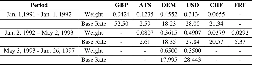
Table 2.2 Basket Composition, Currency Weights, and Base Rates across Periods

Period GBP ATS DEM USD CHF FRF

Jan. 1,1991 - Jan. 1, 1992 Weight 0.0424 0.1235 0.4552 0.3134 0.0655 -Base Rate 52.50 2.59 18.23 28.00 21.34 -Jan. 2, 1992 – May 2, 1993 Weight - 0.0807 0.3615 0.4907 0.0379 0.0292

Base Rate - 2.61 18.35 27.84 20.57 5.37 May 3, 1993 - Jun. 26, 1997 Weight - - 0.6500 0.3500 -

-Base Rate - - 17.995 28.443 -

-Weights sum up to 1 and represent relative importance of particular currency in the balance of payments. Base rates are constant over respective period.

imposed on the basket was set at ± 0.5%. The CNB managed to keep the index of the basket within the band during all three periods. The index was held on average at 0.9999, 1.0011, and 0.9952 for the respective periods. However, minor mismanagements occurred as can be seen in Figure 2.3 that shows the evolution of the currency basket index over the entire period.

Figure 2.3 Evolution of the Currency Basket Index

0.993 0.995 0.997 0.999 1.001 1.003 1.005 1.007

1 55 109 163 217 271 325 379 433 487 541 595 649 703 757 811 865 919

Sequential Trading Days

Index Value

2.3 Process underlying exchange rate movement

2.3.1 Theoretical background

Many economic and especially financial variables reflect the stylized facts attributed to Mandelbrot (1963). These are: (1) unconditional distributions have thick tails, (2) variances change over time, and (3) large (small) changes tend to be followed by large (small) changes of either sign. These stylized facts are especially appealing in the context of high frequency financial data such as exchange rates and stock prices.

international asset portfolios, and the pricing of options on foreign currencies. The opening of new emerging markets in Central Europe has led to interest in the behavior of exchange rates of these economies since they broaden frontiers to international investments. To know the statistical properties and to define the behavior of the particular currency may lower the risk involved in international financial activity.

The fat tails of the exchange rates distributions imply increased uncertainty, and this feature attracts attention. In order to account for leptokurtosis, two different explanations were suggested in literature, namely by Friedman and Vandersteel (1982). One idea suggests that the rates are independently drawn from a fat tail distribution that is fixed over time. The other view favors distributions that vary over time. Hsieh (1988) found a strong statistical evidence to discriminate between the two competing theories. His evidence points to the rejection of the first hypothesis because of changing means and variances of daily rates. This feature can be best described by accounting for the conditional autoregressive heteroskedasticity in modeling the variance that was first introduced by Engle (1982).

emerge from both motives mentioned above. The consistent monetary policy of the central bank with respect to the stable index is therefore imperative in order to produce mathematically consistent semi-fixed exchange rates. Fortunately, this is the case for the Czech koruna.

Milhøj (1987) modeled the distribution of daily deviations of the U.S. Dollar to Special Drawing Rights (SDR) using a simple ARCH model. SDR has been a composite of currencies since July 1, 1974. However, the U.S. Dollar is not pegged to this basket and thus such a modeling does not involve semi-fixed exchange rate. Therefore, the exchange rate of the Czech koruna to other currencies represents an interesting modeling challenge.

2.3.2 Autoregressive conditional heteroskedasticity

The original ARCH model framework of Engle (1982) suggests that current volatility depends on past squared innovations in order to explain the tendency of large residuals to cluster together. Bollerslev (1986) extended the framework into a generalized autoregressive conditional heteroskedasticity model (GARCH) where current volatility depends not only on past squared residuals but also on lagged autoregressive component, e.g. lagged own variances. By deriving residuals εt from an

underlying process, which are conditioned by the information set Ωt, a

GARCH(p,q) process is given by )

, 0 ( ~

| 2

1 t

t

t N σ

ε Ω − (2.2)

with conditional autoregressive variance specified as

∑

∑

= −

= −

+ +

= q

j

j t j p

j

j t j t

1 2

1 2

2 _{ω α ε β σ}

σ . (2.3)

Conditional variance may be denoted by ht in the part of the literature. We

feel that use of 2

t

type that has been used to describe financial data volatility is the generalized specification GARCH(1,1).

Whether the ARCH process described above is present in the data can be detected by subsequent tests. In order to remove any linear structure in the data, an autoregressive filter is applied. Each series is modeled as an autoregressive process of the form

t i t

r +ε

∑

10

1 = i i 0

t = a + a

r (2.4)

where εt is independently and identically distributed (iid). The Akaike

Information Criterion (AIC) method of Akaike (1974) was employed to determine the appropriate number of lags.

Table 2.3 shows the results of two independent test performed on residuals from the mean equation (AR(10)) to detect presence of an ARCH process described above. A Lagrange-multiplier test suggested by Engle (1982), tests a null hypothesis that no ARCH process is present in the data. The values of LM(10) are distributed according to the chi-squared distribution with 10 degrees of freedom and the null hypothesis can be decisively rejected at any confidence level for all six rates.

Table 2.3 Testing for conditional heteroskedasticity and serial correlation

Statistics GBP ATS DEM USD CHF FRF

LM(10) 77.00 114.44 82.34 51.06 77.49 96.01 Q(10) 0.3536 0.0964 0.0936 0.282 0.0104 0.1987 Q2_{(10) 110.05 156.94 130.32 64.97 94.24 135.09} Skewness -1.441 -0.404 -0.674 0.326 -0.179 -0.854 Kurtosis 14.600 2.394 3.523 1.815 2.561 6.474

LM: Lagrange multiplier test by Engle (1982), Q: Ljung-box test against higher order serial correlation by Ljung-Box (1978), χ2 _{critical value at 1% level with 10 d.f. is 23.21}

Despite the fact that the tests were performed using the autoregressive process with 10 lags, the results of both tests are not sensitive to any particular choice of lags, as they were replicated for control purpose with different structures.

The values of the unconditional sample kurtosis exceed a normal value in the case of three currencies. This fact, along with the results of previous tests, shows that an autoregressive process appears to account for the serial correlation properties of the daily data. However, it does not adequately describe the heteroskedasticity or the large kurtosis present in the daily rates. The next step is to employ an ARCH model with conditionally distributed errors and daily dummy variables in both conditional mean and conditional variance equations.

2.4 Conditional variance

2.4.1 Modelling

Brock, Hsieh, and LeBaron (1993), p. 130, point out that a prevalent view in literature is that exchange rates follow a random walk. However, no strong statistical evidence has emerged to confirm or refute this view so far. Research done with exchange rates and security prices uses random walk as well as different univariate processes. When taking into account a basket pegged character of the exchange rates in the data set, a possibility of a specific underlining process cannot be overlooked.

determine the appropriate number of lags. AR(10) structure was also the efficient way to filter the data so that the model yielded residuals free of autocorrelation and seasonality as well. To capture plausible changes of the distribution in different days during a business week, appropriate day-of-the-week dummy variables were employed. The specification of the model resulted into the following mean equation

t t HO t TH t WE t TU t MO i t d d d d d r ε γ γ γ γ γ + + + + + + +

∑

where, | ~ (0 , 2)

t

1 σ

ε_t Ω_t− D , and a conditional variance equation

t HO t TH t WE t TU t MO t d d d d d , 5 , 4 , 3 , 2 , 1 2 1 -t 2 1 2 t

φ φ φ

φ φ βσ αε ω σ + + + + + + + + = ₋ (2.6)

where dMO,t, dTU,t, dWE,t, dTH,tare dummy variables for Monday, Tuesday,

Wednesday, and Thursday, and dHO,t is the number of holidays (excluding

weekends) between successive business days.

The restrictions on the parameters in the variance equation require that

ω > 0, α ≥ 0, and β ≥ 0. Further, when α + β < 1, then the unconditional

variance is finite and stationarity is ensured by not having unit root as shown by Bollerslev (1986).

Estimation of the model is performed by using a log-likelihood function of the form

(

)

(

)

2 1 2 2

1 ln /

t t t

L = − σ − ε σ . (2.7)

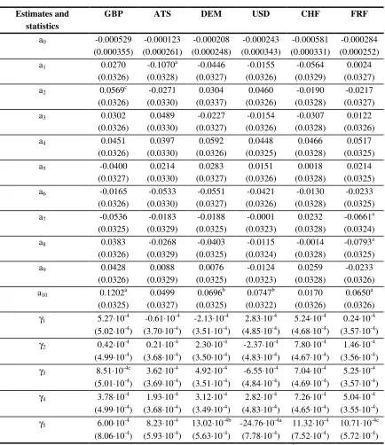
Table 2.4 Estimating the mean equation for GARCH(1,1) r_t a a r_{i t} d

i j j jt t

= + ₋ + + = =

∑

∑

GBP ATS DEM USD CHF FRF

a0 -0.000529 (0.000355) -0.000123 (0.000261) -0.000208 (0.000248) -0.000243 (0.000343) -0.000581 (0.000331) -0.000284 (0.000252) a1 0.0270

(0.0326) -0.1070a (0.0328) -0.0446 (0.0327) -0.0155 (0.0326) -0.0564 (0.0329) 0.0024 (0.0327) a2 0.0569c

(0.0326) -0.0271 (0.0330) 0.0304 (0.0337) 0.0460 (0.0326) -0.0190 (0.0328) -0.0217 (0.0327) a3 0.0302

(0.0326) 0.0489 (0.0330) -0.0227 (0.0327) -0.0154 (0.0326) -0.0307 (0.0328) 0.0122 (0.0326) a4 0.0451

(0.0326) 0.0397 (0.0330) 0.0592 (0.0326) 0.0448 (0.0325) 0.0466 (0.0328) 0.0517 (0.0325) a5 -0.0400

(0.0327) 0.0214 (0.0330) 0.0283 (0.0327) 0.0151 (0.0326) 0.0018 (0.0328) 0.0214 (0.0325) a6 -0.0165

(0.0326) -0.0533 (0.0330) -0.0551 (0.0327) -0.0421 (0.0326) -0.0130 (0.0328) -0.0233 (0.0325) a7 -0.0536

(0.0325) -0.0183 (0.0329) -0.0188 (0.0325) -0.0001 (0.0323) 0.0232 (0.0328) -0.0661a (0.0324) a8 0.0383

(0.0326) -0.0268 (0.0329) -0.0403 (0.0325) -0.0115 (0.0324) -0.0014 (0.0328) -0.0793a (0.0325) a9 0.0428

(0.0326) 0.0088 (0.0329) 0.0076 (0.0325) -0.0124 (0.0323) 0.0259 (0.0328) -0.0233 (0.0326) a10 0.1202a

(0.0325) 0.0499 (0.0327) 0.0696b (0.0325) 0.0747b (0.0322) 0.0170 (0.0326) 0.0650a (0.0326)

γ1 5.27⋅10-4

(5.02⋅10-4₎

-0.61⋅10-4 (3.70⋅10-4₎

-2.13⋅10-4 (3.51⋅10-4₎

2.83⋅10-4 (4.85⋅10-4₎

5.24⋅10-4 (4.68⋅10-4₎

0.24⋅10-4 (3.57⋅10-4₎

γ2 0.42⋅10-4

(4.99⋅10-4₎

0.21⋅10-4 (3.68⋅10-4₎

2.30⋅10-4 (3.50⋅10-4₎

-2.37⋅10-4 (4.83⋅10-4₎

7.80⋅10-4 (4.67⋅10-4₎

1.46⋅10-4 (3.56⋅10-4₎

γ3 8.51⋅10-4c

(5.01⋅10-4₎

3.62⋅10-4 (3.69⋅10-4₎

4.92⋅10-4 (3.51⋅10-4₎

-6.55⋅10-4 (4.84⋅10-4₎

7.04⋅10-4 (4.69⋅10-4₎

5.25⋅10-4 (3.57⋅10-4₎

γ4 3.78⋅10-4

(4.99⋅10-4₎

1.93⋅10-4 (3.68⋅10-4₎

3.12⋅10-4 (3.49⋅10-4₎

2.82⋅10-4 (4.83⋅10-4₎

7.26⋅10-4 (4.65⋅10-4₎

5.04⋅10-4 (3.55⋅10-4₎

γ5 6.00⋅10-4

(8.06⋅10-4₎

8.23⋅10-4 (5.93⋅10-4₎

13.02⋅10-4b (5.63⋅10-4₎

-24.76⋅10-4a (7.78⋅10-4₎

11.32⋅10-4 (7.52⋅10-4₎

10.71⋅10-4c (5.72⋅10-4₎

Standard errors are in parentheses. Significantly different from zero at 1% (a_{) , 5% (}b_{) and, 10%(}c_{) level.}

coefficients of lag 10 are highly significant. This confirms the original tests suggesting an AR(10) structure in the data. Lag 10 means exactly two business weeks’ memory of the market.

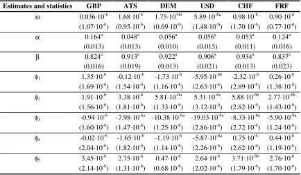
Table 2.5 Estimating conditional variance for GARCH(1,1):

h_t = +ω αε_t−1+βh_t− +

2

1 φ1dMO t, +φ2dTU t, +φ3dWE t, +φ4dTH t, +φ5dHO t,

Estimates and statistics GBP ATS DEM USD CHF FRF

ω 0.036⋅10-6 (1.07⋅10-6₎

1.68⋅10-6 (0.95⋅10-6₎

1.75⋅10-6b (0.69⋅10-6₎

5.89⋅10-6a (1.48⋅10-6₎

0.98⋅10-6 (1.70⋅10-6₎

0.90⋅10-6 (0.77⋅10-6₎

α 0.164a (0.013) 0.048a (0.013) 0.056a (0.010) 0.056a (0.015) 0.053a (0.011) 0.124a (0.016)

β 0.824a (0.016) 0.913a (0.019) 0.922a (0.013) 0.906a (0.021) 0.934a (0.013) 0.837a (0.023)

φ1 1.35⋅10-6

(1.69⋅10-6₎

-0.12⋅10-6 (1.54⋅10-6₎

-1.73⋅10-6 (1.16⋅10-6₎

-5.95⋅10-6b (2.63⋅10-6₎

-2.32⋅10-6 (2.89⋅10-6₎

0.26⋅10-6 (1.38⋅10-6₎

φ2 1.91⋅10-6

(1.56⋅10-6₎

3.38⋅10-6 (1.81⋅10-6₎

5.81⋅10-6a (1.33⋅10-6₎

5.31⋅10-6c (3.12⋅10-6₎

5.88⋅10-6b (2.82⋅10-6₎

2.77⋅10-6b (1.43⋅10-6₎

φ3 -0.94⋅10-6 (1.60⋅10-6₎

-7.98⋅10-6a (1.47⋅10-6₎

-10.38⋅10-6a (1.25⋅10-6₎

-19.03⋅10-6a (2.86⋅10-6₎

-8.33⋅10-6a (2.72⋅10-6₎

-5.90⋅10-6a (1.24⋅10-6₎

φ4 -0.02⋅10-6 (2.04⋅10-6₎

-1.65⋅10-6 (1.82⋅10-6₎

-1.19⋅10-6 (1.14⋅10-6₎

-5.87⋅10-6a (2.26⋅10-6₎

0.75⋅10-6 (2.62⋅10-6₎

0.44⋅10-6 (1.19⋅10-6₎

φ5 3.45⋅10-6

(2.14⋅10-6₎

2.75⋅10-6 (1.31⋅10-6₎

0.47⋅10-6 (0.68⋅10-6₎

2.64⋅10-6 (2.02⋅10-6₎

3.71⋅10-6b (1.79⋅10-6₎

2.76⋅10-6 (1.70⋅10-6₎ Standart errors are in parentheses. Significantly different from zero at 1% (a_{) , 5% (}b_{) and, 10%(}c_{) level.}

Table 2.5 contains results from the iterative estimation of the variance equation, which is of prime interest for the following reason. If a conditional variance changes through time in a predictable way, then the correct modeling of such a variance would yield better estimates of the parameters in the mean equation. It would improve estimates of confidence intervals around the mean forecasts as well. Restrictions put on the coefficients ω, α, and β are satisfied, as well as finite conditional variance condition of α + β < 1. However, Nelson (1991) has shown that even for a region of parameter value beyond this boundary (e.g. α + β > 1) the conditional variance process will be strictly stationary and ergodic.

comparable with those found in literature. All of them are significantly different from zero at 1% level. The magnitude of the lagged variance in all six currencies produce unrefutable evidence of the importance that this lagged term must be included in the equation of the conditional variance.

The sum of the estimated values of α and β amounts on average to 0.937 for all six currencies. This fact might suggest employment of an Integrated GARCH(1,1) model. IGARCH model imposes the restriction α + β = 1 on the coefficients and provides a simpler characterization of exchange rates in question. However, the IGARCH model imposes complete persistence of a shock for infinite time horizon. The covariance stationary GARCH model, on the contrary, implies relatively rapid exponential decay of the shock. Due to the fact that the currency basket peg dilutes external shocks in free rates and other influences proportionately according to the weights, their full impact is eventually damped within a relatively short period of time. This is fully in accordance with the character of the data, and therefore, justifies the use of the GARCH model vs. IGARCH. Further discussion on this subject can be found in Bollerslev and Engle (1993).

Estimates of the day-of-the-week dummy coefficients are fairly small. Despite this, all six currencies show evidence of systematic daily patterns in conditional variance. Similar daily effects were reported by Baillie and Bollerslev (1989) and Hsieh (1988). They are clearly divided into positive and negative effects across days of the week with corresponding daily magnitude levels. Monday, Wednesday, and Thursday show a negative effect while Tuesday, and Holiday show a positive effect. Tuesday’s effect is evident for four currencies and Wednesday’s effect is clearly visible for five of them.

The basket peg causes the exchange rates of koruna to lag one day behind the changes in currencies to which the basket is pegged. This is because free exchange rates at the market in Frankfurt at time (t) are used

to set the currency basket and exchange rates of koruna at time (t+1). Due

When modeling free exchange rates, it would be Monday’s effect that should capture this phenomenon because of the lack of a time lag. The Wednesday’s effect may be understood as a natural correction of the financial markets after a possible over-reacting on accumulated information a day before, as seen on Tuesday in free exchange rate countries.

2.5 Testing the fit of the model

2.5.1 Standard method (Ljung-Box)

The overall fit of the model is assessed by diagnostic tests on standardized residuals zt that are constructed as

t t t

z =ε /σ (2.8)

where εt is the residual of the mean equation (2.5), and σt is a standard

deviation derived from the estimated conditional variance from (2.6). The tests and statistics are shown in Table 2.6.

Means are close to zero and variances tend to unity for the exchange rates residuals. Under these conditions it shows that equations (2.5) and (2.6) are correctly specified. Ljung-Box tests document that first order serial dependency is not present at all. Second order dependence is generally missing as well, however, it is detected at 5% level in standardized residuals for ATS and FRF. Kurtosis dropped for all currencies except USD, though, its decrease in case of GBP and DEM was not large enough to fit into a normal distribution. Kurtosis of ATS, CHF, and FRF decreased sufficiently to fit into normal distribution.

Table 2.6 Tests on standartized residuals

Statistics GBP ATS DEM USD CHF FRF

Mean 0.006 0.008 0.016 0.003 0.009 0.006 Variance 1.117 1.012 1.056 1.129 1.004 1.004 Skewness -1.284 -0.212 0.017 1.370 0.031 -0.547 Kurtosis 12.795 1.028 3.200 12.436 0.885 1.772 nQ(10) 8.427 2.443 2.522 2.918 1.572 4.411 nQ2_{(10) 1.637 20.826 4.246 6.152 11.850 19.144}

2.5.2 BDS test of the fit

The standardized residuals were also examined with a BDS test of Brock, Dechert, Scheinkman, and LeBaron (1996). We refer to this test as the BDS test since this methodology was originally published by Brock, Dechert, and Scheinkman (1987). The BDS test is a nonparametric test of null hypothesis that the data is independently and identically distributed (iid). The technique enables to test for nonlinear dependence and uses the concept of correlation integral employed by Grassberger and Procaccia (1983) to distinguish between chaotic deterministic systems and stochastic systems.

In order to define the correlation integral Cm_,T(ε), let

{ }

time series of lenght T. Then, we form m-dimensional vectors, called m

-histories, m =( _t, _t+1, , _t+m−1)

t x x x

x K . Such _m-dimensional vectors are used to

calculate the correlation integral at embedding dimension m, which is

given by )) 1 ( /( 2 ) , ( ) ( 1 1 1 , =

∑ ∑

= =+ m m

m s m t T t T t s T

m I x x T T

C

m m

ε

ε (2.9)

where T_m =T −m+1, and I_ε(x_tm,x_sm) is an indicator function of event

ε < − − = =

− t₊i s₊i

m j m

i x x

m i x x 1 , , 0supK

.

Thus, the correlation integral measures the fraction of pairs that lie within the tolerance distance e for the particular spatial dimension m.

The correlation integral is used to define the BDS statistics

( )

[

( )

( )

]

( )

m T T

m T

m T C C

BDS _, 2 _{, 1,} / _,

1

−

= (2.10)

where T is the sample size, C_m,T(ε)is the value of a correlation integral or

a number of clustered pairs lying within a particular tolerance distance e at

spatial dimension m, and σ_m,T(ε)is a standard deviation of the statistic

arbitrarily and is chiefly enumerated as a ratio of the sample’s standard deviation.

The BDS test is a nonparametric test of the null hypothesis that the data is independently and identically distributed (iid) against an unspecified alternative. The test enables one to test for nonlinear dependence because it is no affected by linear dependencies in the data. The procedure has power against both deterministic and stochastic systems. The ability of this test to deal with stochastic time series makes its application in modern macroeconomics and financial economics very appealing.

By detecting pairs of histories that cluster together within a specific range ε too often, the BDS test is able to reveal hidden patterns which should not occur in a truly randomly distributed data. A “pattern”, in this case, is defined as an occurrence of two histories that lie within a certain distance ε of each other for different spatial dimensions m. Further

detailed explanation and application of the BDS test can be found in the original paper as well as in numerous studies by Brock and Dechert (1988), Hsieh and LeBaron (1988), Hsieh (1989), Kugler and Lenz (1990), Hsieh (1991), Brock, Hsieh and LeBaron (1993), Kugler and Lenz (1993), Olmeda and Perez (1995), and Kocenda (1996). The software program of Dechert (1987) was used to compute the BDS statistic.

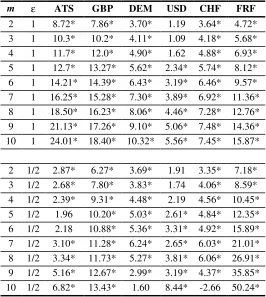
The BDS test is able to reveal hidden patterns in seemingly random numbers. This can be illustrated by results from the BDS test performed on stationary first logarithmic differences to test for the nonlinearity in the data. Results in Table 2.7 support decisive rejection of the hypothesis that logarithmic first differences of the exchange rates are iid for all currencies.

Table 2.7 BDS Test: First Logarithmic Differences

m ε ATS GBP DEM USD CHF FRF

2 1 8.72* 7.86* 3.70* 1.19 3.64* 4.72* 3 1 10.3* 10.2* 4.11* 1.09 4.18* 5.68* 4 1 11.7* 12.0* 4.90* 1.62 4.88* 6.93* 5 1 12.7* 13.27* 5.62* 2.34* 5.74* 8.12* 6 1 14.21* 14.39* 6.43* 3.19* 6.46* 9.57* 7 1 16.25* 15.28* 7.30* 3.89* 6.92* 11.36* 8 1 18.50* 16.23* 8.06* 4.46* 7.28* 12.76* 9 1 21.13* 17.26* 9.10* 5.06* 7.48* 14.36* 10 1 24.01* 18.40* 10.32* 5.56* 7.45* 15.87* 2 1/2 2.87* 6.27* 3.69* 1.91 3.35* 7.18* 3 1/2 2.68* 7.80* 3.83* 1.74 4.06* 8.59* 4 1/2 2.39* 9.31* 4.48* 2.19 4.56* 10.45* 5 1/2 1.96 10.20* 5.03* 2.61* 4.84* 12.35* 6 1/2 2.18 10.88* 5.36* 3.31* 4.92* 15.89* 7 1/2 3.10* 11.28* 6.24* 2.65* 6.03* 21.01* 8 1/2 3.34* 11.73* 5.27* 3.81* 6.06* 26.91* 9 1/2 5.16* 12.67* 2.99* 3.19* 4.37* 35.85* 10 1/2 6.82* 13.43* 1.60 8.44* -2.66 50.24*

BDS follows t-distribution. * indicates 1% significance level (> 2.33).

Table 2.8 BDS tests of nonlinearity: Standardized Residuals GARCH(1,1)

M ε GBP ATS DEM USD CHF FRF

2 1 -1.92 -0.51 -1.10 -0.84 0.79 -0.53 3 1 -2.02* -0.68 -1.37 -1.27 0.75 -1.09 4 1 -1.61* -0.47 -1.37 -1.43* 0.79 -1.23 5 1 -1.78* -0.66 -1.35 -1.50* 0.98 -1.20 10 1 -2.63* -0.64 -1.46 -1.15 0.23 -0.94 2 0.5 -1.95 0.20 -0.51 -1.26 1.01 -0.87 3 0.5 -2.09* 0.21 -1.02 -1.73 0.84 -1.37 4 0.5 -1.71 -0.01 -0.97 -1.80 0.92 -1.38 5 0.5 -2.11 -0.37 -0.93 -1.86 0.27 -1.72 10 0.5 -1.14 4.99 -0.60 -1.72 -4.48 -2.21

Table 2.9 Quantiles of BDS Statistic GARCH(1,1) Standardized Residuals 1000 observations

Quantile m

2 3 4 5 10 N(0,1)

ε=1.0σ

1.0% -1.97 -1.64 -1.42 -1.45 -1.66 -2.33 2.5% -1.69 -1.41 -1.26 -1.20 -1.46 -1.96 97.5% 1.63 1.42 1.32 1.23 1.75 1.96 99.0% 2.01 1.78 1.61 1.51 2.23 2.33

ε=0.5σ

1.0% -2.11 -1.96 -2.09 -2.45 -7.31 -2.33 2.5% -1.84 -1.72 -1.80 -2.05 -6.93 -1.96 97.5% 1.80 1.79 1.92 2.19 16.83 1.96 99.0% 2.29 2.18 2.25 2.69 23.48 2.33

Based on 2000 replications

Source: Brock, Hsieh, and LeBaron (1993), p. 278

Table 2.8 shows the results of the BDS test on standardized residuals. The results can be interpreted with the help of Table 2.9 which contains quantiles of the BDS statistic of standardized residuals from GARCH(1,1) model of exchange rates. The asymmetric distribution was derived by Brock, Hsieh, and LeBaron (1993), p.278, after 2000 replications (the table, however, states values for ε=1 and 0.5 only). For tolerance distance

ε=1 the test reveals no evidence of nonlinear dependence for four currencies: ATS, DEM, CHF, and FRF. However, the critical values are exceeded for spatial dimensions m=3,4,5, and 10 in case of GBP which

shows rather high values for all dimensions in any event, and for m=4, and

5 in case of USD. This indicates the existence of a more complex dimensional structure governing the behavior of these particular rates. In case of USD it is a marginal decision though. A missing nonlinear term is to be added to better the model. At tolerance distance ε=0.5 a nonlinear dependence is not detected in general. The critical value is exceeded at the dimensional level of m=3 in rate of GBP. In no case is the critical value

exceeded at the highest dimensional level. If it were, it would have been for a different reason. As spatial dimension m increases, the number of

of available data, therefore, causes the test to go beyond the statistical range and distortions are likely to occur.

It can be concluded that the model fits all six currencies very well, but GBP requires some nonlinear improvement. Diagnostic tests show that GARCH(1,1) model is capable of accounting for most of the nonlinearity in the particular set of exchange rates.

2.6 Empirical summary

Exchange rates of the Czech koruna to six major currencies evolved relatively stable through the researched period. Due to their dependency on the currency basket, they are of a semi-fixed character. They showed remarkable similarities in behavior and statistical characteristics with those exchange rates that are free to float. This is to be attributed to the consistent policy of the central bank that kept the basket index relatively unchanged within the ± 0.5% band. The exchange rates achieved stationarity after the first logarithmic differencing and were shown not to be identically and independently distributed. Their conditional first moments are linearly independent. However, non-linear dependency was detected in conditional second moments. These facts along with a Lagrange-multiplier test confirmed the presence of an ARCH process in the data.

GARCH(1,1) model was employed to capture the properties of the exchange rates and to model their conditional variance along with the day-of-the-week effects. Mean equation of the model exhibits a strong statistical significance at the tenth lag level which indicates a two business week memory of the market. Variance equation shows highly significant coefficients of lagged residuals and own variance. Altogether it is shown that change in a rate is very closely related to its conditional variance. Strong Wednesday and Tuesday effects uncover a significant sequential responsiveness to the information flow within financial markets.

dependency. However, the latter was detected at 5% level for two currencies. The model accounted for decrease in kurtosis for five currencies, although marginally in two cases.

An advanced nonparametric BDS test revealed existence of nonlinear dependency in exchange rates. Standardized residuals, on the contrary, revealed a lack of such a dependency and become white noise. The only exception is GBP (and marginally USD), where a nonlinear component should be added to improve the model. The particular model accounted for most of the nonlinearity in the data and other nonlinear model is not likely to be able to pick up more of the forecastable structure from a time series.

3

Volatility of exchange rate with change in

fluctuation band

3.1 Altered band

This part extends the analysis of exchange rate and examines the behavior of the Czech koruna when it was pegged to a currency basket under different fluctuation bands. The period of our interest starts after the monetary separation of the Czech and Slovak republics in the beginning of 1993 until the end of 1996. It offers a different angle of application of generalized autoregressive conditional heteroskedasticity to analyze a currency movement. In chapter 2 we outlined monetary environment in which the exchange rate of the koruna evolved since 1991.

Most importantly we stated that the koruna could not be openly traded for several years and its full was instituted convertibility on October 1, 1995. This measure meant that the koruna could be traded for foreign exchange without restrictions by both companies and citizens. However, this step was not paired with any kind of change in the exchange rate regime itself.

increased volatility of the koruna. Whether this is true is addressed in the following analysis that starts with data description.

3.2 Data

The data consists of daily midpoint exchange rates of the Czech koruna (CZK) to six major currencies from January 4, 1993 to December 31, 1996. The data was supplied by the Czech National Bank (CNB), Prague. The rates of foreign currencies in terms of the Czech koruna are: Deutsche Mark (DEM), U.S. Dollar (USD), British pound (GBP), Canadian dollar (CAD), Japanese yen (JPY), and Swedish kron (SEK). The six major currencies were selected for this study because the majority of them are quite important in international trade (USD, GBP, JPY), and some of them are included in the currency basket to which the Czech koruna was pegged (USD, DEM). Another reason is that they represent a set of currencies that are governed by different exchange rate regimes: from a real free float (USD, CAD, JPY) to a more limited float or interlinked peg (DEM, SEK, GBP). A significant reason for analyzing CAD, JPY, GBP, and SEK is the fact that these currencies were not in any formal way associated with the composition of the basket during the researched period.

There are a total of 1016 daily observations for each currency. The data are not stationary but represent a first order integrated process. A further analysis is performed on the rate of change of respective exchange rates calculated as a percentual change between two consecutive business days. Such a transformed time series exhibits the usual mean close to zero and skewness and kurtosis far from normality, as one would expect in the case of high frequency financial data.

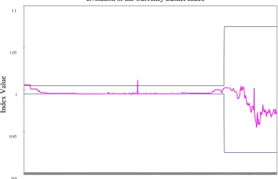
the basket within the band during both periods. However, minor incidents of mismanagement occurred, as can be seen in Figure 3.1. Again, it should be stressed that the index, calculated from daily midpoint exchange rates, serves only as an illustration of how it evolved over time.

Figure 3.1

Evolution of the Currency Basket Index

0.9 0.95 1 1.05 1.1

1 31 61 91 121 151 181 211 241 271 301 331 361 391 421 451 481 511 541 571 601 631 661 691 721 751 781 811 841 871 901 931 961 991 Sequential Trading Days

Index Value

3.3 Leverage effect

information set Ωt, a GARCH(p,q) process is given by ) , 0 ( ~ | 2 1 t t

t N σ

ε Ω ₋ with conditional autoregressive variance specified as

∑

∑

2 _{ω α ε β σ}

σ . (3.1)

Research done with exchange rates and security prices uses random walk as well as different univariate processes to model underlying movement in the data. When taking into account the basket pegged character of the exchange rates in the data set and having performed several tests, we opted for an autoregressive process to model the underlying movement in the data. The number of lags was determined to be 1, 1, 3, 1, 1, and 2 for DEM, USD, GBP, CAD, JPY and SEK, respectively. The mean equation was specified as

t i t

r +ε

∑

t = a + a

r (3.2)

where, | ~ (0, 2)

1 t

t

t D σ

ε Ω − .

In order to analyze volatility of the koruna the following concept was introduced. A change in volatility is analyzed with the use of a phenomenon known as a “leverage effect,” which is the negative correlation between volatility and past returns. Following the parametrization of Glosten, Jagannathan, and Runkle (1993) and its application by Engle and Ng (1993) and Hamilton and Susmel (1994), the variance equation was specified as

2 1 -t 1 2 1 2 1

2 _{ω α ε β σ ξ ε}

σt = + ⋅ t− + ⋅ t− + ⋅dt− ⋅ (3.3)

where dt₋₁ is a dummy variable that is equal to zero if εt−1 >0, and equal

to unity if εt₋₁ ≤0. The leverage effect predicts that ξ >0. The restrictions on the parameters in the variance equation require that ω >0,

0

≥

shown by Bollerslev (1986). The above specification yields the GARCH-L(1,1) model that is estimated later.

The leverage effect was analyzed in stock price movements. For example, in the case of equities, Black (1976) and Nelson (1991), among others, argued that a stock price decrease tends to increase subsequent volatility by more than would a stock price increase of the same magnitude. In the case of the exchange rate, the leverage effect represents the fact that a decrease in the price of a foreign currency in terms of the koruna, or the koruna’s appreciation, would tend to increase the subsequent volatility of the koruna more than would a depreciation of an equal magnitude. Despite the fact that holding foreign exchange is, in terms of risk, similar to holding equities, literature dealing with the “leverage effect” in the context of exchange rate fluctuation is still lacking.

While the value of the statistically significant leverage coefficient ξ

indicates the magnitude of the leverage effect, the sign implies its direction. A positive value of the coefficient ξ indicates an increase, and a negative coefficient indicates a decrease in subsequent volatility of the exchange rate. By comparing values and signs of statistically significant leverage coefficients for a particular exchange rate in the two separate periods of narrow and wide fluctuation bands, it is possible to comment on the effect of the fluctuation band change on the koruna’s volatility.

3.4 Leverage effect empirics in exchange rate

An estimation of the model was performed by using a log-likelihood function of the form

(

(

)

)

2 1 2 2

1 ln /

t t t

L = − σ − ε σ . The maximum

likelihood estimates were obtained by using a numerical optimization algorithm described by Berndt, Hall, Hall, and Hausman (1974). The results from the estimation are presented in Table 3.1 and Table 3.2 for narrow and wide fluctuation band periods respectively.

insignificant in the first period but highly significant in the later one. The second period dominates the whole process and the number of lags in the AR model is kept the same in both periods for the sake of consistency.

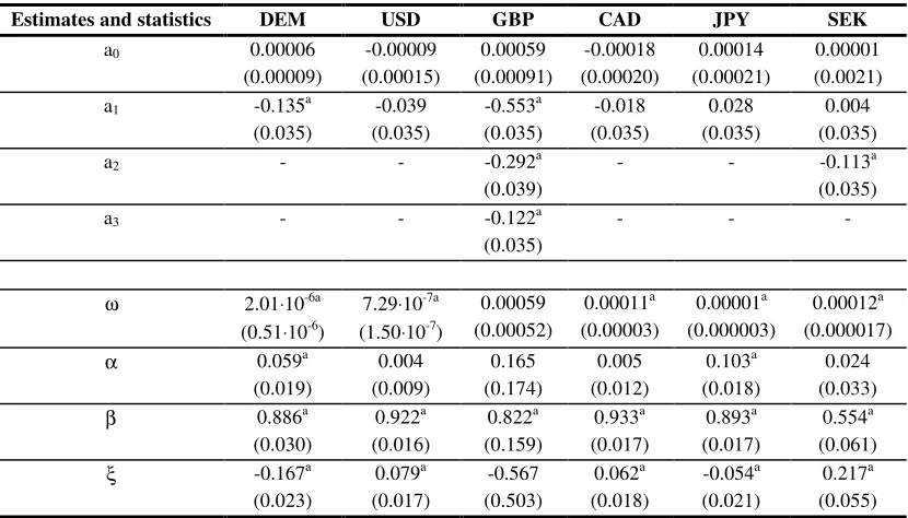
Table 3.1

Estimating GARCH-L (1,1): First (Narrow Band) Period

Estimates and statistics DEM USD GBP CAD JPY SEK

a0 0.00006

(0.00009) -0.00009 (0.00015) 0.00059 (0.00091) -0.00018 (0.00020) 0.00014 (0.00021) 0.00001 (0.0021) a1 -0.135a

(0.035) -0.039 (0.035) -0.553a (0.035) -0.018 (0.035) 0.028 (0.035) 0.004 (0.035)

a2 - - -0.292a

(0.039)

- - -0.113a

(0.035)

a3 - - -0.122a

(0.035)

- -

-ω 2.01⋅10-6a

(0.51⋅10-6₎

7.29⋅10-7a

(1.50⋅10-7₎

0.00059 (0.00052) 0.00011a (0.00003) 0.00001a (0.000003) 0.00012a (0.000017) α 0.059a

(0.019) 0.004 (0.009) 0.165 (0.174) 0.005 (0.012) 0.103a (0.018) 0.024 (0.033) β 0.886a

(0.030) 0.922a (0.016) 0.822a (0.159) 0.933a (0.017) 0.893a (0.017) 0.554a (0.061) ξ -0.167a

(0.023) 0.079a (0.017) -0.567 (0.503) 0.062a (0.018) -0.054a (0.021) 0.217a (0.055) Standard errors are in parentheses. Significantly different from zero at 1% (a_{) , 5% (}b_{) and, 10%(}c_{) level.}

In the case of the variance equation, coefficients of constant ω are small and mostly insignificant. Estimates of lagged squared residuals α and lagged variance β are generally large and comparable with those found in the literature. Nearly all of them are significantly different from zero at 5 or 10% level; however, 1% level significance predominates. The magnitude of the lagged variance in most of the currencies provides irrefutable evidence of the importance of including this lagged term in the equation of the conditional variance.

dollar starts with a relatively small positive coefficient for the first period and ends up with an almost equal coefficient of the negative sign in the second one. This represents a significant change in the behavior of this exchange rate as well as the tendency for the volatility to decrease during the wide band period as in the case of the Deutsche mark.

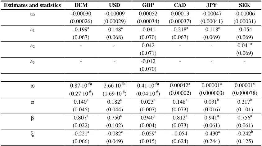
Table 3.2

Estimating GARCH-L (1,1): Second (Wide Band) Period

Estimates and statistics DEM USD GBP CAD JPY SEK

a0 -0.00030

(0.00026) -0.00009 (0.00029) 0.00052 (0.00034) 0.00013 (0.00037) -0.00047 (0.00041) -0.00006 (0.00031) a1 -0.199a

(0.067) -0.148a (0.068) -0.041 (0.070) -0.218a (0.067) -0.118c (0.069) -0.054 (0.069)

a2 - - 0.042

(0.071)

- - 0.041a

(0.069)

a3 - - -0.012

(0.070)

- -

-ω 0.87⋅10-6a

(0.27⋅10-6₎

2.66⋅10-5a

(1.69⋅10-6₎

0.41⋅10-6a

(0.04⋅10-6₎

0.00042a (0.00002) 0.00001a (0.000003) 0.00001c (0.000078) α 0.140a

(0.045) 0.182a (0.044) 0.023a (0.007) 0.148a (0.073) 0.031b (0.016) 0.217b (0.101) β 0.807a

(0.022) 0.750a (0.102) 0.940a (0.004) 0.812a (0.073) 0.941a (0.061) 0.756a (0.061) ξ -0.221a

(0.066) -0.082c (0.049) -0.059a (0.015) -0.054 (0.624) -0.430a (0.244) -0.242b (0.125) Standard errors are in parentheses. Significantly different from zero at 1% (a_{) , 5% (}b_{) and, 10%(}c_{) level.}

later. This indicates a considerable decrease in volatility for this exchange rate.

The results of the analysis clearly indicate that allowing for the wider fluctuation band resulted in a decrease in volatility of the key currencies (DEM and USD), as well as of two other ones (JPY and SEK). An analysis of the other two currencies (GBP and CAD) is unfortunately precluded by the lack of statistical significance associated with the leverage effect coefficient in the broad or wide band periods respectively. One possible explanation might be the fact that the key currencies (DEM and USD), being a part of the currency basket, affect themselves directly. Their movements actually counteract each other because their influences represented by weights in the basket must be strictly balanced in order to keep the basket index constant. However, the wide fluctuation band allows relatively far deviations from this target. This is empirically documented by the evolution of the index that stayed almost entirely within the appreciation part of the fluctuation band during the wide band period (see Figure 3.1).

The currencies that are not part of the basket are affected indirectly by a simple mechanical calculation of their exchange rate for each respective day. Their diminished volatility associated with a wider fluctuation band then goes against conventional wisdom, which is documented in some previously published work. Flood and Rose (1995) claim that “fixed exchange rates are less volatile than floating rates, but the volatility of macroeconomic variables such as money and output does not change very much across exchange rate regimes.” Hasan and Wallace (1996) argue that using long-term data “real exchange rate volatility is greater for flexible exchange rate periods than for fixed-rate periods.”

3.5 Brief summary

The central point of the analysis is how the change in the fluctuation band of the index affected volatility of the exchange rate.

By allowing for a wider fluctuation band, the CNB let the exchange rate fluctuate more freely, thus reducing its potential nominal stability. Because of the fact that the currency basket was introduced to keep a relatively stable nominal exchange rate and limit its volatility, a further implication is that allowing for a wider fluctuation band should lead to more pronounced movements and increased volatility of the koruna.

4

Intratemporal links among interest and exchange

rates

4.1 Basic facts

Chapters 2 and 3 presented some economic and institutional background of the exchange rate regime that governed the behavior of the Czech koruna from the early 90’s. Since exchange rate regime is an important element in the overall monetary policy of each country, it transfers a great deal of influence into the financial market. Such an influence is often likely to be indirect via

interest rates. Our goal in this part is to assess the money market in the Czech Republic and to study the interactions between short and long interest rates, and specifically a lead-lag relationship. In particular, we will study linkages between interest rates, as well as exchange rates, and compare the results of the periods before 1997 with those in the year when the country experienced financial crisis. Despite the fact that the turbulence in the mid of 1997 was officially labeled as a financial crisis, in the view of what happened on a global scale in 1998 such term should be understood with caution.

As we said before, former Czechoslovakia officially started its economic transformation in 1991. The temporary anchor of an exchange rate regime based on a currency basket peg with a new level of base rates was introduced in 1991 as a part of overall transformation strategy. Czech koruna emerged after the split of the country into two independent nations followed shortly by the formal monetary separation. Over the years several important changes took place. First, the Czech National Bank (CNB) changed the composition of the basket on January 2, 1992, and then on May 2, 1993. From the latter date on, the basket was composed of the US dollar and the Deutsche mark at a ratio of 35:65. Second, there was a

change of the fluctuation band. The band imposed on the basket was originally set at ± 0.5%. It was widened on February 28, 1996, to allow the index to fluctuate by ± 7.5%, while the exchange rate was still kept within the fixed regime. Previous chapters dealt with this subject in detail.

During the period from 1991 to 1996 the koruna evolved in a relatively stable manner. The stability was interrupted in 1997.

From the very beginning of 1997 the exchange rate started to appreciate significantly. In the middle of February it reached a local maximum of 5.5% above a central parity, and from then on it steadily depreciated. At first the fall was not very sharp and the rate even became steady in the beginning of May. A strong speculative pressure had emerged by the middle of May. CNB fought the speculative attacks for roughly two weeks with the help of foreign exchange interventions and with a sharp increase in interest rates. Then on May 26, 1997, the CNB abandoned the fixed exchange rate regime and let the koruna float freely with some unspecified tie to the Deutsche mark. The koruna immediately devalued by 12-13%. This dive stopped quite quickly, and subsequently the koruna strengthened and moved into the lower range of the original parity.

The devaluation of the koruna acted as a natural pro-export feature and hurt the economy only mildly. The sharp increase in interest rates was the damaging factor, instead. The CNB ceased performing repo operations on May 15, 1997, and set a floating repo rate, which was dependent on the current market situation. The rates rose slightly. On May 16, 1997, the CNB increased the lombard rate from 14 to 50%, and during the next week it started to lower market liquidity with a 45 and later 75% repo rate. As a result of such strict monetary policy, short-term interest rates on the inter-bank market reached an unbelievable 200% and even peaked above 400%. Commercial banks were cut off from liquidity and acted accordingly. Tied to the subsequent appreciation of the currency, interest rates decreased but did not reach original levels.

for the evolution of links among key interest rates. The bonds among interest rates tended to evolve in a weak economic sense. They naturally changed from 1993, when a modern banking sector emerged in the country. In 1996 these links were found to be quite independent. The peaceful evolution lasted till the beginning of 1997. Then turbulence started to sweep the entire industry and to erode the original arrangements. It is not our purpose to discuss whether the interest rates were correctly or incorrectly set during the crisis. Rather we would like to take the interest rate settings as exogenous shocks and analyze what their impact was. The great exogenous shocks might have great effect on links among interest rates at the inter-bank market and the position of its leading rate. Similar links are expected to exist between the exchange rate and interest rates.

4.2 Vector autoregresive analysis of lead-lag relationship

A usual vector autoregressive process (VAR) specification is

t m t Y m A t

Y A A t

Y = ₀ + ₁⋅ ₋₁ +...+ ₋ +Ε , (4.1)

where Y is a list of macroeconomic variables. A VAR is a non-structural

model which simply estimates how variables are related to their lagged values over time. VAR models have been used extensively, in particular in macroeconomic forecasting. Several authors give a strong critique of structural models, arguing that VAR works better for forecasting and for policy evaluation (see Litterman (1979) and Sims (1980) among others). On the other hand, VAR specification represents a reduced form of a structural model.

al. (1993) among others. A similar approach has been used to test interrelations between the cash market and stock index futures by Chan (1992) and Kawaller et al. (1987), to mention a few.

The described model fits our goal of studying the efficiency of the newly established inter-bank market in the Czech Republic. The interactions between short and long interest rates, and specifically a lead-lag relationship, are our general interest. In particular, we intend to study linkages between interest rates, and later between exchange rates and interest rates.

If the inter-bank market is efficient, then arbitrage and base trading will maintain the correct pricing relationship. This lead-lag relationship can be attributed to several specific factors of the Czech inter-bank market: the unsettled character of the new market, the low volume of trade for some maturities, and institutional design. While strong bilateral links support the hypothesis of market integration, a unilateral link leads to market segmentation and arbitrage opportunities.

To test such a hypothesis we use the tool of Granger causality. We say that “{x_t} Granger causes {y_t},” when the lagged values of x_t have an

explanatory power in regression of y_t on lagged values of y_t and x_t. The

Granger causality is then tested via an autoregressive representation:

    +           =     t t t t t t y x L d L c L b L a y x δ ε ) ( ) ( ) ( ) ( . (4.2)

For a review of alternative tests see Geweke et al. (1983).

Because disturbances are serially uncorrelated, the direction of causality between {xt} and {yt} can be turned into a standard test of whether b(L)=0

and/or c(L)=0. The test of the hypothesis “{x_t} Granger causes {y_t}” is

equivalent to the test of the restriction b(L)=0. Similarly, the opposite

direction of causality can be tested via the restriction c(L)=0.

We applied Hsiao's (1981) two-step approach to determine the length of the lag structure. The linkages between inter-bank interest rates were examined in the context of the following models:

t i t k

i i i

t k

i i

t X Y

X =α + α ∆ + β ∆ +ε

∆ ₋

= −

=

∑

∑

1 1

0 (4.3)

t i t k

i i i

t k

i i

t Y X

Y =χ + χ ∆ + δ ∆ +ν

∆ ₋

= −

=

∑

∑

1 1

0 , (4.4)

whereX_t and Y_t denote interest rates associated with different maturity.

For each maturity the proper pair of lag lengths (k₁,k₂) and (k₃,k₄)

were specified using a search method over a range of lag lengths from 1 to 10. The choice of the optimal lengths was based on standard information criteria of Akaike (1969), Hannan-Quinn (1979), and Schwarz (1978). Thorton and Batetten (1985) show the sensitivity of the causal relationships (links) to the chosen number of lags. In particular, it is necessary to test whether both series are cointegrated. Such testing is extensively illustrated by the standard methodology developed by Engle and Granger (1987).

Therefore, we did several robust checks, using the number of lags recommended by different information criteria. Moreover, we used six and seven lags of both the dependent and independent variables to test for market linkages. In all cases, we obtained the same results. Because the error terms were not autocorrelated and cointegration was not rejected for any equation, we tested the lead-lag relationship between the interest rates by stating the following hypothesizes:

H0 : βi =0 for all i, which means that there is no link from maturity Y to

X

and

H0 : δi =0 for all i, which means that there is no link from maturity X to

4.3 Data

All the data we used were provided by the CNB. We used daily exchange rates of the koruna in terms of the US dollar and the Deutsche mark. Further we used daily interest rates for different maturities. One is the

Prague Interbank Offer Rate (PRIBOR); the other is the Prague Interbank Bid Rate (PRIBID). Both rates were used in price quotations

for: one day, one week, two weeks, one month, two months, three months, six months, nine months, and one year. We are aware of the fact that a one day rate is known to behave rather strangely sometime. However, we included this rate to cover the entire range of interest rates on the interbank market.

There was a total of 1131 observations, which were divided according to years in the following manner: 1993 with 229 observations, 1994 with 247 observations, 1995 with 245 observations, 1996 with 245 observations, and 1997 with 165 observations. The years from 1993 to 1996 cover 12 months each. The data for 1997 covers a period of nine months.

As one might expect, the data are the first order integrated process. The analysis is therefore performed on the changes in exchange and interest rates between two consecutive business days.

4.4 Intratemporal linkages

4.4.1 Overall inter-bank performance

Figure 4.1 One Day Offer Rate on the Prague Inter-bank Market: January 3, 1993 to September 30, 1997

It is very useful to look at the spread, which is defined as the difference between offer and bid rate. The spread is often used as a proxy to measure the degree of stability on the market. Figure 4.2 shows the evolution of short-term interest rate spreads on the inter-bank market from January 3, 1993, to May 16, 1997, just immediately prior to the crisis. It can be concluded that the period before the crisis was characterized by a notable decline in spreads. This can be translated into low uncertainty in and low volatility of the money market.

0.00 10.00 20.00 30.00 40.00 50.00 60.00 70.00 80.00 90.00 100.00 110.00 120.00 130.00 140.00 150.00 160.00 170.00 180.00 190.00 200.00