Munich Personal RePEc Archive
Targeting the Poor in Vietnam using a
Small Area Estimation Method
Nguyen Viet, Cuong
10 August 2005
Online at
https://mpra.ub.uni-muenchen.de/25761/
Nguyen Viet Cuong1
Abstract
To estimate the poverty rate at the commune level, the Ministry of Labor, Invalids and
Social Affairs firstly collects information on households’ income per capita, and compares
their income with a defined poverty line. A household is identified as a poor one if their
income per capita is below the poverty line. Then, the poverty rate of a commune is
simply the ratio of the defined poor households in that commune. This method can raise
questions about the quality of the collected data on income. This paper examines the
quality of expenditure data collected in this simple way. It is found that the expenditure
data collected in the simple way are considerably lower than expenditure data collected
using detailed questionnaires. Thus collection of expenditure or income data using simple
questionnaires tends to underestimate the actual expenditure or income. For poverty
targeting in small areas such as communes or districts, this paper suggests the application
of this small areas estimation method.
Keywords: Poverty, the poor, poverty targeting, poverty mapping, small area estimation
JEL classification: I31, I32, O15
1
Researcher in National Economics University, Hanoi, Vietnam.
1. Introduction
Poverty reduction is a major development policy in Vietnam. The Government of Vietnam
has set up a target of reducing the poverty rate from 26% in 2005 to 15% in 2010
(MOLISA, 2005)2. In order to support the poor, the first step is to locate where the poor
live and to identify who the poor are. The Ministry of Finance will allocate more resources
to the poorest communes, and then the Ministry of Labor, Invalid and Social Affairs
(MOLISA) will identify who the poor are to provide supports. Officially, MOLISA
collects information on households’ income per capita, and then compares their income
with a defined poverty line. A household then is identified as a poor one if their income
per capita is below the poverty line. The poverty rate of a commune is simply the ratio of
the defined poor households in that commune. This method can raise a question about the
quality of the collected data on income. As is known, the income of a household can come
from many sources and varies from one month to another. A quick interview using short
questionnaires would result in income data with a large measurement error. However
identifying the poor throughout the country using long interview with detailed
questionnaires is not feasible, since it is extremely costly.
Estimation of poverty rates in small areas is proposed by Elbers et. al. (2003) and
Hentchel et. al. (2000). They combine population censuses and household surveys to
estimate poverty indices at the district and commune levels. Population censuses cover the
whole population and collect information on basic household characteristics such as
demography and housing, but not household income and expenditure. In contrast,
household surveys often collect data on both household characteristics and expenditures
(or also income) using very detailed questionnaires. Household surveys, however, are
sample surveys and representative for national or regional levels. To estimate the poverty
rate for small areas, an equation of expenditure (or income) is firstly estimated using a household survey, and then it is applied in a population census to predict expenditure
(income) using information on household characteristics and the poverty rate. Once the
poverty rate at the commune level can be estimated, the poor households in the commune
2
can be identified by alternative methods such as through commune meetings or by using
income data from MOLISA.
The most recent poverty map that used the small area estimation method was
produced in 2003 by (Minot, Baulch, and Epprecht, 2003). They combine data from the
Vietnam Living Standard Survey in 1998 (VLSS 1998) and data from the Population and
Housing Census in 1999 to estimate the poverty rates at a small level, i.e. province,
district and commune. In 2006 the Vietnam Census on Agriculture, Rural Areas and
Aquaculture will be conducted, which allows for possibility to update the poverty map for
the rural areas of Vietnam.
This paper has two main objectives. The first is to investigate whether collection of
data on expenditure using quick and simple questionnaires can yield reliable expenditure
data. The second is to test how the small area estimation works in the recent Vietnam
Living Household Standard Survey (VHLSS) in 2004. If the method works well, there
will be the possibility of updating the poverty map for Vietnam using the 2006
Agricultural Census and the 2006 VHLSS.
This paper is divided into 5 sections. The second section introduces data sources
used in the paper. The third section examines the measurement error in expenditure data
collected using the simple method. The fourth section presents results from the small area
estimation. Finally, some conclusions are drawn in the final section.
2. Data Sources
The first data source is the Vietnam Household Living Standard Survey (VHLSS) that was
conducted by the General Statistical Office of Vietnam (GSO) in the year 2004. The
survey collected information on household characteristics including basic demography,
employment and labor force participation, education, health, income, expenditure, housing, fixed assets and durable goods, the participation of households in the most
important poverty alleviation programs. The full household sample of the VHLSS covered
the 45000 households, of which 9000 households were asked for detailed information on
very detailed questionnaires. Small and detailed items on expenditure and income are
collected, and then aggregated into the expenditure and income per capita. The sample of
9000 households is used in this research. The sample is representative for the whole
country and 8 geographic regions.
The second data source is from a pilot survey conducted by the Institute of Labor
Science and Social Affairs (ILSSA) of MOLISA. This survey was conducted in early
2005. The survey collected data on household characteristics, expenditure and income of
households in 9 communes in 4 provinces: Tuyen Quang, Thanh Hoa, Quang Nam, and
An Giang. Expenditure and income are collected using simple questionnaires. It should be
noted that all households in each commune are quickly surveyed by a “questionnaires part
A1” to remove the rich households from the sample. Basically, the Part A1 uses short and
quick questionnaires to find households who have high value assets such as cars or boats,
or have stable sources of high income. These households can be regarded as rich ones and
are removed from the sample. In addition, in some communes the interviewers do not
collect information from households who are considered very poor by the “questionnaires
part A2”. The remaining households which are considered are the poor and near-poor
ones. These households are interviewed using “questionnaires part B”. This research uses
data on these remaining households collected based on this “questionnaires part B”. The
number of households in this sample is 4526.
3. Measurement Error in Expenditure Data of the Pilot Survey
3.1. Methodology
It is often argued that collection of expenditure data using simple survey methods can
underestimate the actual expenditure. This section examines the accuracy of expenditure data of the pilot survey by comparing these data with expenditure data collected in the
2004 VHLSS. The pilot survey collects expenditure data using very simple questionnaires,
while the 2004 VHLSS collects expenditure data using detailed questionnaires and
benchmark, and expenditure data of the pilot survey will be considered accurate if they are
close to the expenditure data of the 2004 VHLSS.
The aim of this test is to estimate the average difference between expenditure per
capita of households in the 2004 VHLSS and expenditure per capita of households in the
pilot survey after household characteristics variables are controlled for.
Assume that expenditure per capita, denoted by yi is a function of observed
variables X and unobserved variables ε :
i i
i X
y =α+ β+ε . (1)
We pool two samples of VHLSS and the pilot survey, and denote D as a binary
variable indicating whether a household is from the pilot survey. Equation (1) can be
expressed as follows:
yi =α+Xiβ+Diθ+εi. (2)
If there is no difference in expenditure data between the two surveys, the coefficient of
variable D is not statistically significant. In this paper, we estimate equation (2) by OLS
and quantile regression. We also estimate the coefficient D by a matching method with the
distance metric of propensity score. The idea of the matching method is to find similar
households between the 2004 VHLSS and the pilot survey. This can be regarded as a
non-parametric method that is used to estimate the parameter θ.
3.2. Empirical Results
Before pooling the two samples, we need to make them comparable to avoid the problem
of sample selection bias. It should be noted that the pilot survey did not cover some rich
households in all communes nor some very poor households in 5 communes in two
provinces. Thus to make the two samples more comparable, the procedure to remove the
rich households using the questionnaires Part A1 is applied to the VHLSS 2004. As a
In addition, only households who are in 4 communes of two provinces “Tuyen
Quang” and “An Giang” are kept for the analysis, since one did not apply the
questionnaires Part A2 to exclude very poor households in these communes. The
procedure is rather arbitrary; thus we cannot apply this method to the VHLSS 2004 to
exclude the very poor households so that all samples of the pilot survey can be used for
this expenditure comparison analysis.
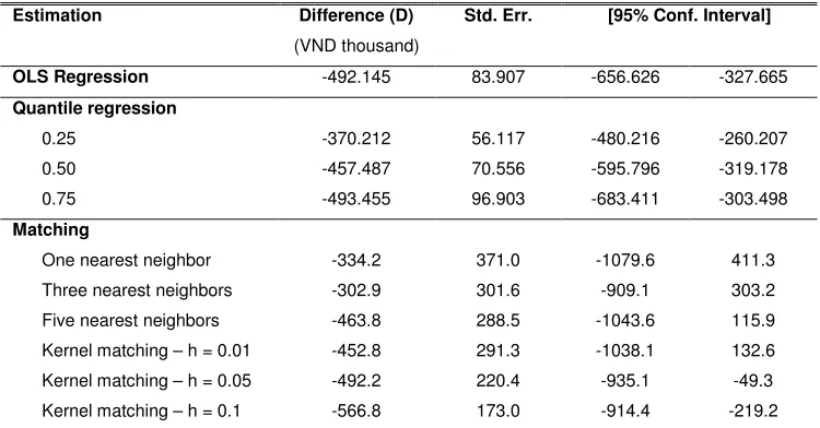
Table 1 presents the estimates of the difference in expenditure per capita between
the VHLSS 2004 and the pilot survey controlling for some observed variables that are
correlated with the expenditure. Explanatory variables include urban and regional dummy
variables, commune characteristics, household composition, education of household
members, education and employment of household head and head’s spouse, housing
characteristics, and assets. Households included in the analysis are restricted to low
expenditure samples.3 Estimation from the regressions shows that expenditure data in the
pilot survey are statistically significantly lower than expenditure data in the 2004 VHLSS.
The non-parametric methods also produce a similar trend, but some of the estimates are
[image:7.612.116.491.457.653.2]not statistically significantly at 5%.
Table 1: Average difference in expenditure per capita between the 2004 VHLSS and the pilot
survey: regression and propensity score matching estimations
Estimation Difference (D)
(VND thousand)
Std. Err. [95% Conf. Interval]
OLS Regression -492.145 83.907 -656.626 -327.665
Quantile regression
0.25 -370.212 56.117 -480.216 -260.207
0.50 -457.487 70.556 -595.796 -319.178
0.75 -493.455 96.903 -683.411 -303.498
Matching
One nearest neighbor -334.2 371.0 -1079.6 411.3
Three nearest neighbors -302.9 301.6 -909.1 303.2
Five nearest neighbors -463.8 288.5 -1043.6 115.9
Kernel matching – h = 0.01 -452.8 291.3 -1038.1 132.6
Kernel matching – h = 0.05 -492.2 220.4 -935.1 -49.3
Kernel matching – h = 0.1 -566.8 173.0 -914.4 -219.2
Standard error in the matching method is estimated using bootstrap with 200 replications
Source: Estimation form the 2004 VHLLS and pilot survey
3
Thus, the collection of expenditure data using simple questionnaires and quick
interview is more likely to underestimate the actual expenditure. The consumption basket
has a large number of small items, and detailed questionnaires help people remember
these small items in their consumption. These results suggest that income data collected
by MOLISA might not be reliable in estimating the poverty rate at the commune or
district level. An alternative way to estimate poverty indexes in small areas is to combine
a census and a household survey using the method of small area estimation.
4. Small Area Estimation Method
4.1. Methodology
Poverty is widely measured by three Foster-Greer-Thorbecke poverty indices, which can
all be calculated using the following formula (Foster, Greer and Thorbecke, 1984):
=
− =
q
i
i
z y z n P
1
1 α
α , (3)
where yi is a welfare indicator (consumption expenditure per capita in this paper) for
person i, z is the poverty line, n is the number of people in the sample population, q is the
number of poor people, and α can be interpreted as a measure of inequality aversion.
When α = 0, we have the headcount index H which measures the proportion of
people below the poverty line. When α = 1 and α = 2, we have the poverty gap PG which
measures the depth of poverty, and the squared poverty gap P2 which measures the
severity of poverty, respectively.
Poverty indices are often estimated using data from household surveys. In
Vietnam, during the period 2000-2010, the GSO conducted Vietnam Household Living
Standard Surveys (VHLSS) once every two years. However samples of VHLSS are often
small, and results cannot be representative in small areas such as communes or districts. In
contrast, population censuses cover large sections of the population but do not collect
from censuses either. The method of “small area estimation”, developed by Elbers et. al.,
(2003), and Hentschel et. al., (2000), combines a household survey and a population
census to estimate a poverty headcount index (H) for small areas. The main idea is to
estimate an expenditure equation from a household survey, and use this equation to predict
expenditure for households in a census given the households’ characteristics. Once
predicted expenditures are available, poverty rate can be estimated at small areas.
In Vietnam, the most recent poverty map to use the small area estimation method
was produced in 2003 by Minot et. al., 2003. They estimate poverty indices at the
province, district and commune levels using the Vietnam Living Standard Survey of 1998
and the Population and Housing Census of 1999. In this paper, we examine how the
method works using data from the 2004 VHLSS.
The method of small area estimation involves the following three steps:
Step 1: Select common variables from the household survey and a population census.
These variables will be used in a regression of expenditure, and therefore should be
correlated with expenditure.
Step 2: Run regression of expenditure on selected variables using data from the household
survey:
i i i X
y )= ' β+ε
ln( , (4)
where:
- yi is the real per capita consumption expenditure of household i
- Xi’ is a 1xk vector of household characteristics of household i
- is a kx1 vector of estimated coefficients
- i is a random disturbance term distributed as N(0, )
The list of variables may be revised for the final equation.
Step 3: Apply this equation to the population census to predict the expected probability
that household i is poor:
− Φ = σ β σ β i C i i X z X P
where:
- Pi is a variable taking a value of 1 if the household is poor and 0 otherwise
- z is the poverty line
- is the cumulative standard normal function
- XiC household characteristics for household i from the census
Then the poverty rate for an area can be estimated according to Elbers et al (2003):
= − Φ = N i C i i
C z X
M m X P E 1
2] ln
, , | [ σ β σ
β (6)
where:
- mi is the size of household i
- M is the total population of the area in question
- N is the number of households in the area
To estimate the poverty gap index PG, and the poverty severity index P2, we
employ the method proposed by Minot, et. al., 2003 to estimate the cumulative
distribution of the expenditure per capita in the absence of the VBSP credit. This is done
by changing the poverty line from the lowest expenditure per capita to the highest
expenditure per capita in the sample. The estimated cumulative distribution is then used to
estimate the poverty indexes PG and P2 (in the state of no-credit from the program).
In this paper, we will estimate the poverty indices in two ways. In the first, poverty
indices are estimated directly from expenditure data of the 2004 VHLSS. These estimates
can be regarded as a benchmark, since they use the observed data on expenditure. The
second way applies the method of small area estimation to obtain the poverty indices. If
the small area estimation functions well in the 2004 VHLSS, it is expected that the two
ways of estimation will produce close estimated poverty indexes.
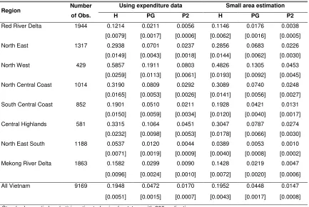
The poverty indices can be easily estimated from expenditure data using equation (3). The
left panel of Table 1 presents poverty indices of 8 regions in Vietnam that are estimated
using observed expenditure data. It is shown that there is large variation in the poverty
indices between the regions. The poverty rate is lowest in the North East South, at around
5.4%. The region with the highest level poverty is the North West, in which 58.6% of the
[image:11.612.91.524.243.534.2]people are below the poverty line.
Table 2: Poverty indexes estimated by the small area estimation method in VHLSS 2004
Region Number
of Obs.
Using expenditure data Small area estimation
H PG P2 H PG P2
Red River Delta 1944 0.1214 0.0211 0.0056 0.1146 0.0176 0.0038
[0.0079] [0.0017] [0.0006] [0.0062] [0.0016] [0.0005]
North East 1317 0.2938 0.0701 0.0237 0.2856 0.0683 0.0226
[0.0149] [0.0043] [0.0018] [0.0144] [0.0062] [0.0030]
North West 429 0.5857 0.1911 0.0803 0.4826 0.1305 0.0453
[0.0259] [0.0113] [0.0061] [0.0193] [0.0092] [0.0045]
North Central Coast 1014 0.3190 0.0809 0.0292 0.3089 0.0740 0.0248
[0.0165] [0.0053] [0.0026] [0.0141] [0.0056] [0.0027]
South Central Coast 852 0.1901 0.0510 0.0211 0.1928 0.0421 0.0131
[0.0150] [0.0059] [0.0034] [0.0120] [0.0040] [0.0017]
Central Highlands 581 0.3315 0.1064 0.0451 0.3047 0.0787 0.0274
[0.0232] [0.0098] [0.0053] [0.0178] [0.0066] [0.0030]
North East South 1188 0.0537 0.0120 0.0044 0.0389 0.0053 0.0010
[0.0071] [0.0019] [0.0009] [0.0040] [0.0008] [0.0002]
Mekong River Delta 1863 0.1582 0.0299 0.0090 0.1428 0.0219 0.0047
[0.0096] [0.0024] [0.0010] [0.0072] [0.0020] [0.0006]
All Vietnam 9169 0.1948 0.0472 0.0170 0.1952 0.0448 0.0147
[0.0051] [0.0015] [0.0007] [0.0043] [0.0017] [0.0008]
Standard error (in bracket) is estimated using bootstrap with 200 replications Source: Estimation form the 2004 VHLLS and pilot survey
The estimates of the poverty indices using the small area estimation method are
presented in the right of Table 2. In this method, the first step is to construct the
expenditure equation using the VHLSS 2004. In expenditure models, the dependent
variables are often in logarithmic form, since this enables them to better fit the data. The
main priority in constructing the expenditure model is to select appropriate explanatory
variables taking into account that the number of explanatory variables should not be too
detailed information on households as household surveys. Explanatory variables include
urban and regional dummy variables, commune characteristics, household composition,
education of household members, education and employment of household heads and
head’s spouses, housing characteristics, and assets. The selection of explanatory variables
is similar to the procedure of backward selection in stepwise regression. Variables are
dropped when they have a P-value higher than 0.1.4
It is found that with the exclusion of the North West region, this method of small
area estimation yields estimates of headcount ratios which are very close to those based on
the collected data for all regions and the whole country. One reason for the large
difference in poverty estimates in the North West is the small number of observations:
there are 429 household observations in the 2004 VHLSS sample. Thus, a caution should
be exercised when estimating poverty in areas with small numbers of observations. An
another reason for the difference might be that the standard error tends to be higher for
observations where values of the characteristic variables X are far from the sample mean
values. In this paper we estimate a single equation of expenditure for the whole sample.
The North West is the poorest region in the sample data, and predicted expenditures for
this region can have large standard errors. When applying this method in a new census,
different expenditure equations can be estimated for different regions or large provinces.
5. Conclusions
To support the poor, it is necessary to identify who the poor are and where they live. To
classify the poor we need the information on welfare indicators such as income or
expenditure. Collection of accurate data on expenditure (or income) using detailed
questionnaires is unrealistic for a large sample. A traditional method is to collect
expenditure (or income) using short and simple questionnaires. However, it is found that
the expenditure data collected by the simple questionnaires tends to be lower than the
actual expenditure.
4
To estimate the poverty rate in small areas such as districts or communes, the
method of small area estimation can be used. For reliable estimation, the number of
observations in small areas should not be too small, and different models of expenditure
References
Elbers, C., Lanjouw, J. and Lanjouw, P. (2003). Micro-level estimation of poverty and
inequality. Econometrica 71 (1): 355-364.
Hentschel, J., Lanjouw, J., Lanjouw, P. and Poggi, J. (2000). Combining census and
survey data to trace the spatial dimensions of poverty: a case study of Ecuador. World
Bank Economic Review Vol. 14(1): 147-65
Minot, N., Baulch, B., and Epprecht, M. (2003). Poverty and Inequality in Vietnam:
Spatial Patterns and Geographic Determinants. Final report of project “Poverty Mapping