Temperature Fluctuations in a Rectangular Nanochannel

http://dx.doi.org/10.4236/jbnb.2015.63011

How to cite this paper: Fornés, J.A. (2015) Temperature Fluctuations in a Rectangular Nanochannel. Journal of Biomaterials and Nanobiotechnology, 5, 117-125. http://dx.doi.org/10.4236/jbnb.2015.63011

Temperature Fluctuations in a Rectangular

Nanochannel

José A. Fornés*

Departamento de Fsica Aplicada I, Facultad de Ciencias Físicas, Universidad Complutense, Madrid, Spain Email: [email protected]

Received 10 April 2015; accepted 24 May 2015; published 27 May 2015

Copyright © 2015 by author and Scientific Research Publishing Inc.

This work is licensed under the Creative Commons Attribution International License (CC BY).

http://creativecommons.org/licenses/by/4.0/

Abstract

We consider an incompressible fluid in a rectangular nanochannel. We solve numerically the three dimensional Fourier heat equation to get the steady solution for the temperature. Then we set and solve the Langevin equation for the temperature. We have developed equations in order to deter-mine relaxation time of the temperature fluctuations, τT = 4.62 × 10−10 s. We have performed a

spectral analysis of the thermal fluctuations, with the result that temporal correlations are in the one-digit ps range, and the thermal noise excites the thermal modes in the two-digit GHz range. Also we observe long-range spatial correlation up to more than half the size of the cell, 600 nm; the wave number, q, is in the 106 _m−1 _{range. We have also determined two thermal relaxation}

lengths in the z direction: l1 = 1.18 nm and l2 = 9.86 nm.

Keywords

Nanochannels, Temperature Fluctuations, Random Heat Flow, Thermal Relaxation, Temporal and Spatial Correlations

1. Introduction

drophobic channel walls with electrokinetic effects and Naviers slip condition [8]. Also optical detection of sin-gle molecule in solution, inside submicrometer channels has become more and more important [9]-[11]. A fun-damental understanding of the transport phenomena (fluid and energy) in nanofluidic channels is critical for systematic design and precise control of such miniaturized devices towards the integration and automation of Lab-on-a-chip devices. T.-C. Kuo et al. [12] investigated molecular transport through nanoporous nuclear-track- etched membranes with fluorescent probes by manipulating applied electrical field polarity, pore size, mem-brane surface functionality, pH, and the ionic strength. Y. Liu et al. [13] studied ion size and image effect on electrokinetic flows with the results that ion size had significant effects on electrokinetic flows in nanosystems. Stepišnik and Callaghan [14] [15] applied the NMR modulated gradient spin-echo method (MGSE) [16] to measure the velocity correlation and the diffusion coefficient of fluid in microcapillary. F. Detcheverry and L. Bocquet developed an analytical description of the thermally induced fluid motion. They estimated several physical quantities under thermal fluctuations [17].

We believe that the knowledge of temperature correlations and the relaxation of the fluctuations could be im-portant for a better understanding of channel fluid phenomena and design.

In the present work, we consider an incompressible fluid at rest in a nanochannel, in which the transfer of energy takes place entirely by thermal conduction. In order to report the temperature fluctuations, we set and solve the Langevin equation for the temperature.

2. Thermal Conduction

The heat flow is related to the temperature gradient by the Fourier law. However, when fluctuations are present, there also appear spontaneous energy fluxes disconnected from this gradient. The “random” contributions to the dissipative heat flux will be designed by g. Then, the fluctuating phenomenological law read [18]:

T κ

= − +

q ∇ g (1)

κ

(

1 1

)

W m⋅ − ⋅K− is the thermal conductivity.

The equation of heat transfer is particularly simple for an incompressible fluid at rest, in which the transfer of energy takes place entirely by thermal conduction (see [18] [19])

2

p

T

T

t χ ρc

∂ _{= ∇ +} ⋅ ∂

g

∇

(2)

p

c

(

1 1

)

J kg⋅ − ⋅K− is the specific heat at constant pressure and χ

(

m2⋅s−1

)

is the thermometric diffusivity, defined as

.

p

c

κ χ

ρ

= (3)

The last term is the fluctuations contribution in accordance to Equation (1). We observe, in this case, the tem- perature equation is decoupled from the density and velocity equations.

2.1. Random Heat Flow

The correlations among the components of the random heat flow in an incompressible fluid are [18]:

( ) (

, ,

)

0 if

i k

g r t g r′ ′t = r≠r′ (4)

( ) (

)

2

(

) (

)

, , 2 .

i k B ik

g r t g r′ ′t = k T κδ δ t−t′ δ r−r′ (5)

Performing the derivative, we obtain:

( ) (

, ,

)

2

₍

_{) (}

1

_{) (}

₎

2 .

i k

B ik k

g t g t

k T x x t t

x κδ δ δ

−

′ ′ ∂

′ ′ ′

= − − − −

∂

r r

r r (6)

(6) transform

( )

2 ₂

( ) ( )

1 1

, 2

k B kk

g r t = k T κδ ∆V − ∆t − (7)

( )

(

) ( ) ( )

2

1 1 1

2 ,

2 .

k

B ik k

k

g t

k T x V t

x κδ − − − ∂ = − ∆ ∆ ∆ ∂ r (8)

Deriving inside the bracket, we obtain

( )

( )

, 2

( )

1

( ) ( )

1 1

, k .

k B ik k

k

g t

g t k T x V t

x κδ − − − ∂ = − ∆ ∆ ∆ ∂ r

r (9)

Approximating

( )

( )

1 2 2

, ,

k k

g r t ∼ g r t inside the bracket of Equation (9), we obtain from Equations (7), (9)

( )

, 1 2

₍

₎

1 2

_{( )}

1

_{( ) ( )}

1 2 1 2

2 .

k

B k

k

g t

k T x V t

x κ − − − − ∂ = − ∆ ∆ ∆ ∂ r (10)

Then we can write

( )

, 1 2

₍

₎

1 2

₍

_{) ( )}

1 1 2

_{( )}

2 .

k

B k

k

g t

k T x V t

x κ ζ

− − − ∂ = − ∆ ∆ ∂ r (11)

If ∆xk is the same for the three coordinates, we obtain,

(

)

1 2

( ) ( )

1 1 2

( )

1 2

3 2 kBκ T xk V ζ t

− −

−

⋅ = − ×g ∆ ∆

∇ (12)

or

( )

ATζ t

⋅ =g

∇ (13)

with

(

) ( )

1/ 2 5 6 1 2

3 2 B

A= − × − k κ ∆V − (14) where we have used ∆ = ∆xk

( )

V 1 3, and ξ

( )

t is the thermal noise, defined by its statistical properties, namely,

( )

t 0

ξ = (15)

( ) ( )

t t

(

t t

)

ξ ξ ′ =δ − ′ (16)

i.e., the correlation time of the noise is zero.for this term. Then

( )

( )

1

d d .

t t t t

t t

AT AT

t t t W t

t t ζ t

+∆ +∆

⋅ = ⋅ = = ∆

∆

∫

∆

∫

∆

g g

∇ ∇ (17)

We used the definition of the Wiener’s process (see [20] [21]), where ∆W t

( )

is the “Wiener’s increment”.

2.2. Langevin Equation for the Temperature

To numerically solve Equation (2) we need to perform a discretization. This is achieved by multiplying both members by dt and performing the integration in the interval

(

t t, + ∆t

)

, namely,

2 2 2

2 2 2

1

d d

t t t t

p

t t

T T T

T t t

c

x y z

χ ρ +∆_{∂ ∂ ∂ } +∆ ∆ = _ + + _ + ⋅ ∂ ∂ ∂  

∫

∫

∇ g (18)

( )

2 2 2

2 2 2

p

T T T AT

T t W t

c

x y z

χ

ρ

∂ ∂ ∂ 

∆ = _ + + _∆ + ∆

∂ ∂ ∂

  (19)

where in the last term of the former equation we have used Equation (17).

At the limit ∆ →t dt the mean values at the RHS of the former equation can be reemplace by the instanten-ous values, this means that the overline on the expressions can be omitted, while ∆W t

( )

=dW t

( )

. From the developments in the appendix we need to recall here that the “Wiener’s process” dW t

( )

is just a Gaussian stochastic process of width σ =

( )

dt 1 2. Then, at each pass of the integration we have to draw dW t

( )

and nor- malize the result properly. That is to say, if RG is an aleatory number, with Gaussian distribution, centered in

0

G

R = and width 1. In MATLAB, RG=randn; consequently we can write

( ) ( )

1 2

dW t = dt RG. To conclude

the discretization process, Equation (19) is transformed in the corresponding Euler’s equation giving the tem-poral evolution of the temperature, namely,

2 2 2

1 1 2

2 2 2 d d .

n n n n

n n

G p

T T T AT

T T t t R

c

x y z

χ

ρ

+ _{= +} ∂ ₊∂ ₊∂  ₊

 _{∂ ∂ ∂} 

  (20)

Defining B A

( )

ρcp 1

−

= , we have

(

) ( )

1 2 5 6 1 2 3 2 . B p k V B c κ ρ − − − × ∆

= (21)

Then the temperature relaxation time, will be

( )

2

( )

5 3 2 2 . 9 p T B c V B k ρ τ κ − ∆

= = (22)

From now on the averages ... are over the realizations of the stochastic process. A first basic quantity of interest is the average temperature current in the long-time limit (i.e, after transients due to initial conditions have died out)

( )

: lim t

T t T

t →∞ t

∂ ₌

∂ (23)

where

( )

1

( )

R R R

T t T t

N

=

∑

(24)

where NR is the number of realizations.

2.3. Numerical Method

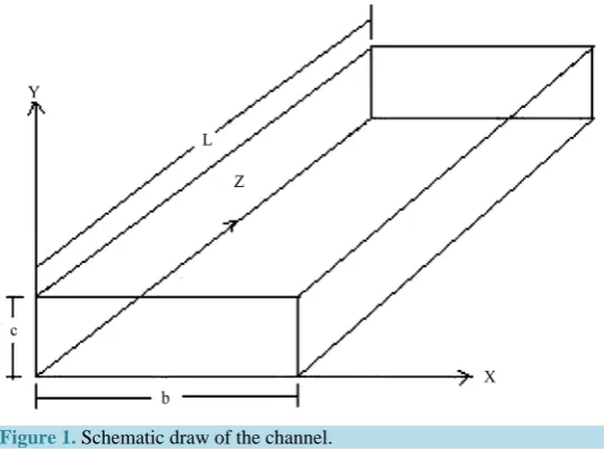
We consider a fluid in a rectangular cross section nanochannel, Figure 1, with the size along the x axis (width b) and the size along the y axis (height c). The length of the channel is denoted by L. The boundary conditions are:

(

0, ,

)

(

, ,

)

(

, 0,

)

(

, ,

)

293 K

T y z =T b y z =T x z =T x c z = , T x y

(

, , 0

)

=298, T x y L

(

, ,

)

=293. We have

consi-dered equal increments in the three coordinates, dx=dy=dz, consequently, we have to comply with the nu-merical stability condition, known as CFL (Courant-Friedrichs-Lewy), which reads for our case:

2 d 1 3 , 2 d t x

χ ≤ (25)

considering the equal sign, we obtain for the ratio of time to spatial increments

d d

.

d 6

t t

[image:5.595.178.450.84.286.2]

Figure 1. Schematic draw of the channel.

Then the discretization for the temperature equation envolving fluctuations, will be

(

)

1

, , , , 1, , 1, , , 1, , 1, , , 1

1 2 , , 1 , , , ,

1 6

6 d .

n n n n n n n

i j k i j k i j k i j k i j k i j k i j k

n n

i j k i j k i j k G

T T T T T T T

T T BT t R

+

− + − + +

−

= + + + + +

+ − ⋅ +

(27)

The first step of the numerical procedure is the choice of the volume dV, and the corresponding spatial grid step dx, in our case dx=dV1 3. Next, the corresponding time step dt is evaluated from the CFL condition,

( )

2 1

d d

6

t x

χ

= . In selecting the number of temporal steps the code needs to run, Nt, we consider the temporal

interval of 2τT, enough for dying out of the transients due to initial conditions. Hence,

1

2 d

t T

N = τ × t− , where 2

T B

τ ₌ −

. In our simulation, we have dV =10−27m3, then dx=

( )

dV 1 3 =10−9m, dt=1.44 10× −12s, 10

4.62 10 s T

τ _{= ×} −

, and Nt =606, b=200 nm, c=50 nm, L=800 nm,

3 3

10 kg m

ρ_{= ⋅} −

,

3 2

10 N s m

η₌ − _{⋅ ⋅} −

, cp 4183 J kg K

(

)

1

−

= ⋅ ⋅ , χ=1.4564 10× −7 m2⋅s−1, κ=0.6092 W⋅

(

m K⋅

)

−1, the corres-ponding grid is 50 200 800× × points.

To numerically evaluate the steady state solution, Ti j k0, , , we proceed as follows: First we initialize our working grid by setting all the matrix components of the temperatures equal to zero, Ti j k, ,  = 0. Next, we solve simultaneously the Equations (27). Every 10 time steps we compute the difference between the actual tempera- tures Ti j k, ,  and the temperature in the previous verification. The maximum of the differences

(

10

)

, , , ,

max t t

i j k i j k

T + T

  − 

    (28) is referred to as the error. Time integration of the equations is stopped when the error is less than a tolerance de-fined at the beginning of the process. We have found that a tolerance tol = 10−9 gives reasonable results for the steady state solution. In this first part of our numerical procedure (namely, the evaluation of the steady state so-lution) we use deterministic equations, i.e. random noise is not considered.

After getting the steady state solution for the temperature, Ti j k0, , . Then we add the corresponding hydrody-namic fluctuation term to the temperature equation, solving this equation over Nt temporal points and Nr

realizations of the stochastic process. Then we analyze the temporal and spatial correlations of the temperature, focusing our study in the center line temperature, TCL.

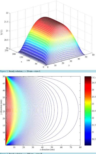
In Figure 2,Figure 3 are shown two views of the steady solution T =T x y

(

,

)

.

3. Results

3.1. Thermal Relaxation

[image:6.595.118.510.84.713.2]

Figure 2.Steady solution, z = 20 nm—view I.

is fitted with two exponential, the corresponding thermal relaxation lengths are l1=1.18 nm and l2 =9.86 nm.

3.2. Autocorrelation Functions for the Central Line Temperature

We have performed spectral analysis of the fluctuations for the central line temperature. As an example of our results, we show in Figure 5(a)the temporal autocorrelation function for the mean (over stochastic realizations) central line (CL) temperature. We observe that the correlation function extends up to 10 ps. Correspondingly, in

Figure 5(b), the Fourier transform of the former autocorrelation function (the spectral density of the mean CL temperature) goes up to the two-digit GHz band.

[image:7.595.142.485.271.491.2]

Regarding the spatial correlation we show in Figure 6(a)the normalized spatial (z axis) autocorrelation func-tion for the mean CL temperature. We can observe that the correlafunc-tion extends over more than half length of the cell, 600 nm, correspondingly, the Fourier transform of this function, Figure 6(b), extends up to wave numbers in the 106 m−1 range. As a validity test of the method we verify that the expectation value TCL obeys the heat conduction equation. The deviations are less than 0.01%. Our present results demonstrate the generic spatially long-range character of nonequilibrium fluctuations.

[image:7.595.88.541.523.690.2]

Figure 4. Temperature profile along y direction for x = b/2 versus the z axis distance to the wall, is fitted with two thermal relaxation lengths.

Figure 5.Temporal autocorrelation functions for TCL , NR=200, Nt=600. (a) Temporal; (b) Fourier transform of the

Figure 6. (a) Spatial autocorrelation function (z axis); (b) Fourier transform of the former spatial autocorrelation function.

4. Conclusion

These such long range correlations appear generically for a wide class of nonequilibrium states [22]. The predic-tions of this phenomenon have been made in a number of contexts, including self-organized criticality [23], li-near response [24], nonequilibrium fluctuating hydrodynamics [25], kinetic theory [26], and stochastic hydro-dynamic [27]-[30].

Acknowledgements

We wish to thank the Fundación Santander-Central-Hispano (Programa de Visitantes Distinguidos UCM) for the support provided.

References

[1] Soong, R.K., Bachand, G.D., Neves, H.P., Olkhovets, A.G., Craihead, H.G. and Montemagno, C.D. (2000) Powering an Inorganic Nanodevice with a Biomolecular Motor. Science, 290, 1555.

http://dx.doi.org/10.1126/science.290.5496.1555

[2] Tsong, T.Y. (2002) Na, K-ATPase as a Brownian Motor: Electric Field-Induced Conformational Fluctuation Leads to Up-Hill Pumping of Cation in the Absence of ATP. Journal of Biological Physics, 28, 309-325.

http://dx.doi.org/10.1023/A:1019991918315

[3] Reisner, W., Pedersen, J.N. and Austin, R.H. (2012) DNA Confinement in Nanochannels: Physics and Biological Ap-plications. Reports on Progress in Physics, 75, Article ID: 106601. http://dx.doi.org/10.1088/0034-4885/75/10/106601

[4] Hou, X., Guoa, W. and Jiang, L. (2011) Biomimetic Smart Nanopores and Nanochannels. Chemical Society Reviews,

40, 2385-2401. http://dx.doi.org/10.1039/c0cs00053a

[5] Lappala, A., Zaccone, A. and Terentjev, E.M. (2013) Ratcheted Diffusion Transport through Crowded Nanochannels.

Scientific Reports, 3, 3103. http://dx.doi.org/10.1038/srep03103

[6] Cheng, L.-J. (2008) Ion and Molecule Transport in Nanochannels. Dissertation of the Requirements for the Degree of Doctor of Philosophy, Electrical Engineering and Computer Science in the University of Michigan.

[7] Zhao, B., Moore, J.S. and Beebe, D.J. (2003) Pressure-Sensitive Microfluidic Gates Fabricated by Patterning Surface Free Energies inside Microchannels. Langmuir, 19, 1873-1879. http://dx.doi.org/10.1021/la026294e

[8] Yang, J. and Kwok, D.Y. (2003) Microfluid Flow in Circular Microchannel with Electrokinetic Effect and Naviers Slip Condition. Langmuir, 19, 1047-1053. http://dx.doi.org/10.1021/la026201t

[9] Eigen, M. and Rigler, R. (1994) Sorting Single Molecules: Application to Diagnostics and Evolutionary Biotechnology.

Proceedings of the National Academy of Sciences of the United States of America, 91, 5740-5747.

http://dx.doi.org/10.1073/pnas.91.13.5740

[10] Goodwin, P.M., Johnson, M.E., Martin, J.C., Ambrose, W.P., Marrone, B.L., Jett, J.H. and Keller, R.A. (1993) Rapid Sizing of Individual Fluorescently Stained DNA Fragments by Flow Cytometry. Nucleic Acids Research, 21, 803-806.

http://dx.doi.org/10.1093/nar/21.4.803

[image:8.595.85.539.79.240.2]

Prospects. Journal of Biotechnology, 86, 181-201. http://dx.doi.org/10.1016/S0168-1656(00)00413-2

[12] Kuo, T.-C., Sloan, L.A., Sweedler, J.V. and Bohn, P.W. (2001) Manipulating Molecular Transport through Nanopor-ous Membranes by Control of Electrokinetic Flow: Effect of Surface Charge Density and Debye Length. Langmuir, 17, 6298-6303.

[13] Liu, Y., Liu, M., Lau, W.M. and Yang, J. (2008) Ion Size and Image Effect on Electrokinetic Flows. Langmuir, 24, 2884-2891.

[14] Stepišnik, J. and Callaghan, P.T. (2000) The Long Time Tail of Molecular Velocity Correlation in a Confined Fluid: Observation by Modulated Gradient Spin-Echo NMR. Physica B: Condensed Matter, 292, 296-301.

http://dx.doi.org/10.1016/S0921-4526(00)00469-5

[15] Stepišnik, J. and Callaghan, P.T. (2001) Low-Frequency Velocity Correlation Spectrum of Fluid in a Porous Media by Modulated Gradient Spin Echo. Magnetic Resonance Imaging, 19, 469-472.

http://dx.doi.org/10.1016/S0730-725X(01)00269-7

[16] Callaghan, P.T. and Stepišnik, J. (1995) Frequency-Domain Analysis of Spin Motion Using Modulated Gradient NMR.

Journal of Magnetic Resonance, Series A, 117, 118-122. http://dx.doi.org/10.1006/jmra.1995.9959

[17] Detcheverry, F. and Bocquet, L. (2013) Thermal Fluctuations of Hydrodynamic Flows in Nanochannels. Physical Re-view E, 88, Article ID: 012106.

[18] Lifshitz, E.M. and Pitaevskii, L.P. (2003) Landau and Lifshitz Course of Theoretical Physics. Volume 9: Statistical Physics, Part 2, Elsevier Butterworth-Heinemann, Oxford.

[19] Landau, L.D. and Lifshitz, E.M. (2004) Landau and Lifshitz Course of Theoretical Physics. Volume 6: Fluid Mechan-ics, Elsevier Butterworth-Heinemann, Oxford.

[20] Gardiner, C.W. (1985) Handbook of Stochastic Methods for Physics, Chemistry and the Natural Sciences. Sprin-ger-Verlag, Berlin. http://dx.doi.org/10.1007/978-3-662-02452-2

[21] Scherer, C. (2005) Métodos Computacionais da Fsica. Editora Livraria da Fsica, USP, São Paulo.(In Portuguese)

[22] Dorfman, J.R., Kirkpatrick, T.R. and Sengers, J.V. (1994) Generic Long-Range Correlations in Molecular Fluids. An-nual Review of Physical Chemistry, 45, 213-219. http://dx.doi.org/10.1146/annurev.pc.45.100194.001241

Kirkpatrick, T.R., Belitz, D. and Sengers, J.V. (2002) Long Time Tails, Weak Localizations, and Classical and Quan-tum Critical Behavior. Journal of Statistical Physics, 109, 373-405. http://dx.doi.org/10.1023/A:1020485809093

[23] Grinstein, G., Lee, D.H. and Sachdev, S. (1990) Conservation Laws, Anisotropy, and “Self-Organized Criticality” in Noisy Nonequilibrium Systems. Physical Review Letters, 64, 1927-1930.

http://dx.doi.org/10.1103/PhysRevLett.64.1927

[24] J. Dufty, in Spectral Line Shapes, p. 1143, edited by B. Wende (W. de Gruyter, NY, 1981); in Long Range Correla-tions, p. 1, edited by J-R. Buchler et al. (Annals NY Acad. Sci., vol. 848,1998).

[25] Lutsko, J.F. and Dufty, J.W. (2002) Long-Ranged Correlations in Sheared Fluids. Physical Review E, 66, Article ID: 041206. http://dx.doi.org/10.1103/PhysRevE.66.041206

[26] Kirkpatrick, T.R., Cohen, E.G.D. and Dorfman, J.R. (1986) Light Scattering by a Fluid in a Nonequilibrium Steady State. I. Small Gradients. Physical Review A, 26, 972-994. http://dx.doi.org/10.1103/PhysRevA.26.972

[27] Schmitz, R. (1988) Fluctuations in Nonequilibrium Fluids. Physics Reports, 171, 1-58.

http://dx.doi.org/10.1016/0370-1573(88)90052-X

[28] Alder, B.J. and Wainwright, T.E. (1970) Decay of the Velocity Autocorrelation Function. Physical Review A, 1, 18-21.

http://dx.doi.org/10.1103/PhysRevA.1.18

[29] Hagen, M.H.J., Pagonabarraga, I., Lowe, C.P. and Frenkel, D. (1997) Algebraic Decay of Velocity Fluctuations in a Confined Fluid. Physical Review Letters, 78, 3785-3788. http://dx.doi.org/10.1103/PhysRevLett.78.3785