TRAINING AND DEVELOPMENT OFARTIFICIAL NEURAL NETWORK MODELS: SINGLE LAYER FEEDFORWARD AND MULTI LAYER FEEDFORWARD NEURAL NETWORK

(1)

ISSN: 1992-8645 www.jatit.org E-ISSN: 1817-3195

VEHICLE COUNTING AND VEHICLE SPEED

MEASUREMENT BASED ON VIDEO PROCESSING

1

HARDY SANTOSA SUNDORO, 2AGUS HARJOKO

1,2

Department of Computer Science and Electronics

Universitas Gadjah Mada, Indonesia

E-mail: [email protected], [email protected]

ABSTRACT

Vehicle counting system and vehicle speed measurement based on video processing are few of systems that utilize digital image processing system as a detector of a moving object such as a vehicle to do the counting and speed measurement. This system is an early stage in the development of Intelligent Transportation System. The methods used in this system are background subtraction with Gaussian Mixture Model (GMM) algorithm and blob detection. Background subtraction method is used because it is a method that can separate foreground and background smoothly and adaptive to the condition of the frame. The blob detection method provide the coordinates in the form of centroid so it will show the movement of the vehicle. System trials conducted on three conditions, namely in the morning, afternoon, and evening. Speed calibration testing parameters obtained with the use of a speed gun. The accuracy of vehicle counting obtained by the evaluation method system by comparing the real situation with the results of the system. The value of the vehicle speed measurement uncertainty obtained by using standard deviation calculations and the combined uncertainty. Vehicle counting accuracy obtained in the morning conditions is 75.69%. Vehicle counting accuracy obatined in the afternoon is 90.50%. Accuracy of counting vehicles obtained 85.31% in the evening. The value of the uncertainty around those conditions is approximately ± 3 km/h

.

Keywords: Intelligent Transportation System, Video Processing, Blob Detection, Background Subtraction, Speed Gun

1. INTRODUCTION

Traffic density becomes very important to know especially in the face of the current number of vehicles passing through a road. A surveyor or observer is usually placed at the curb for counting vehicles passing in front of him. The observer equipped with a tool such as a counter and then press the button counter one by one if a vehicle passed. Implementation of the survey was done manually will lead to human error in the counting process in case the density of the number of passing vehicle, environmental influences or internal condition of the observer itself, resulting in less accurate counting process performed by a surveyor. Besides vulnerable to human error, the counting was done by humans require a separate fee for each implementation so it became less efficient.

Other than passing vehicle on the road, determination of the traffic density required data on the speed of a vehicle crossing the road. By knowing the speed of passing vehicles then we can conclude the estimated density of the road.

Intelligent Transportation System (ITS) is the development of information and communication technologies in the transportation system. ITS is used to improve and streamline mobility, reducing the number of accidents and deaths, as well as preserving the environment.

To achieve these objectives, the following components are identified as the main function of ITS, namely [1]:

1. Maintaining road serviceability and safety

2. Traffic control

3. Travel and user information

4. Demand management

5. Network monitoring

(2)

2. RELATED WORK

Chen, et al. [2] conducted a vehicle counting using blob analysis. The advantages of this system is the accuracy of the calculation reaches 90%. The only drawback of this research is the data retrieval is only done during the afternoon

.

Rahim, et al. [3] calculates the vehicle speed by transforming a 2D image into a 3D image to obtain the position of the vehicle in three-dimensional space. This method consists of image processing, extraction centroid, and tracking. Disadvantages of this system is the algorithm to calculate the speed has not been validated with actual speed so that the accuracy of the estimated speed can not be determined

.

Nurhadiyatna, et al. [4] calculate the speed of a vehicle using CCTV cameras and using the PCA method. Speed calibration use three agents who drove cars and was provided by GPS. The advantages of this system are using CCTV cameras and PCA method. The disadvantages of this system is the accuracy results varied, ranging from 63% to 99.5%.

Sina, et al. [5] developed a research to calculate the number of vehicles and calculate the speed of vehicles with headlight detection method and normalized cross-correlation. The advantages of this system is more focused on methods headlight detection by using light from a vehicle that can be represented as a car.

Pour Mohammad and Dehghani [6] used background subtraction method with estimation based on the intensity of the color brightness. By using this method, moving objects in the image are sequentially detected and the final velocity of the moving object is measured based on geometric calculation. The disadvantage of this system is the accuracy rate of the vehicle reaches ±10% on the degree of uncertainty. The other drawback of this experiment is the data retrieval process that was performed during normal conditions

.

In order to make a better research, we use speed gun for calibration the speed rather than using speedometer. For vehicle counting, system trials conducted on three conditions, namely in the morning, afternoon, and evening so that the results can be seen in any conditions.

3. SYSTEM DESIGN

The design of the vehicle counting system and vehicle speed measurement based video processing includes program design and hardware design using computer vision technology. The design of the program includes the ability to detect the vehicle as

well as calculate and measure the speed of passing vehicles. The design of the hardware is used to retrieve the data video of passing vehicles.

3.1 User Requirement

In the system of counting and measuring vehicle speed, the system requires information about road conditions, particularly the passing vehicles. The resulting outputs of the system are the number of passing vehicles and the vehicle speed of each vehicle are successfully detected. Systems designed using hardware and software as follows:

1. Laptop AMD A6-3400 M APU with Radeon™ HD Graphics 1.40 GHz RAM 4096 MB.

2. Webcam Logitech C525. 3. Camcorder JVC Full HD. 4. Tripod.

5. OpenCV 2.4.3.

6. Speed Gun.

3.2 Data Video Retrieval Scheme

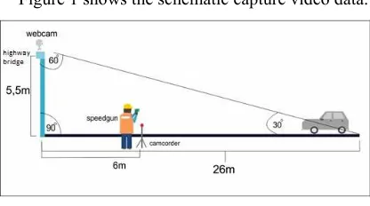
[image:2.612.313.521.423.539.2]

In designing the vehicle counting system and measuring vehicle speed, the technology used is a video image processing via cameras mounted on the highway bridge to monitor the condition of the toll road. Video data used for testing later is a video containing footage of the actual road conditions.

Figure 1 shows the schematic capture video data.

Figure 1: Video Data Retrieval System Scheme

In the process of data retrieval, the webcam is placed on the highway bridge type of concrete with a height of ± 5.5 meters. This height is the standard height of the highway bridge in Indonesia. Concrete highway bridge type was chosen so that when vehicles such as trucks and buses pass, webcam will remain stable.

(3)

ISSN: 1992-8645 www.jatit.org E-ISSN: 1817-3195 The 60º angle determination is based on research

that has been conducted by Li, et al. [7]. According to Li, at 60º angle, the measurement result is more accurate and maximum. The calibration used in this experiment to detect and measure the vehicle speed is in the form of speed gun that was produced by PT. Jasa Marga Persero (Tbk) Branch Semarang, Indonesia. Speed gun is held by a surveyor beside the highway so that when a vehicle passes, the surveyor will be able to "shoot" a passing vehicle with a speed gun to obtain vehicle speed.

3.3 Logic Design Alghorithms

The design of software used in this system is part of image processing system. The input of this system is a video taken with the camera placed above the highway. In this research, the designs of the software are divided into four parts, namely the calibration distance, image preprocessing, vehicle detection and vehicle counting also vehicle speed measurement

.

3.3.1 Calibration distance

Calibration distance is an important part of the measurement process to obtain accurate result. Distance calibration process carried out in accordance with the real conditions on the highway when shooting video data. Distance track is bounded by the ROI (Region of Interest) as a regional area of vehicle counting as well as vehicle speed measurement. Path length caught on camera is then measured manually by using a meter wheel in meters. After that, the next step is the determination of the pixels length on the system based on real conditions.

3.3.2 Image preprocessing

The first stage is taking image using the camera. In this process, the vehicle as the main object captured by the camera in the form of a frame. Then preprocessing procedure is repeated by capturing the frame to produce a video. Video resolution in the system is displayed at the size of 320 x 240 pixels to optimize the image processing computation. The use of measuring resolution of 320 x 240 pixels is also done due to computer limitation.

3.3.3 Vehicle detection

The systems use blob detection method and background subtraction. The use of this method is based on the results of previous studies that have good research final results in accuracy. In addition, blob detection method is used because the method makes it easier to detect objects in the vehicle carefully. Background subtraction method is used because it is a method that can separate moving

objects (foreground) and background smoothly and adaptive to the frame conditions. In general, the steps being taken are as follows:

1. Lane masking

Splitting the part of the road where vehicles are moving in one route.

2. Background elimination

Separating the image of the vehicle from the road to eliminate image noise that may appear as shadows, rain, etc.

3. Blob dan noise filtration

Making the boundary box (blob) of a moving vehicle on the object and removing a small noise to be around the image of the vehicle. 4. Countour labelling

Marking a vehicle that has been detected. 5. Vehicle tracking

First of all, the image obtained will be converted into the format of grayscale. This is done because the monitoring systems are created using algorithms that require grayscale format as input. After that, to eliminate the noise, the image will be transformed to blur.

The road being observed shall be referred to the region of interest (ROI). At ROI, if there are unwanted parts to be detected such as sidewalks and trees, then they will be removed. In order to make the data process more efficient, as well as to avoid other unwanted objecs, the background elimination process is used.

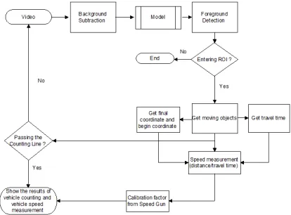
Blob detection is used to detect the shape of the vehicle. All objects that exist in the region of interest will be sought by the edge contours of the vehicle. Blob detection will detect and count the number of vehicles that pass the counting line. Figure 2 shows the flowchart of the vehicle counting system and vehicle speed measurement.

[image:3.612.314.521.549.702.2]

(4)

ISSN: 1992-8645 www.jatit.org E-ISSN: 1817-3195 The centroid value is obtained from blob

detection method which will be used to get mileage and tracking of passing vehicles. By using centroid value, we will know the vehicles’s travel time, by substraction the starting time when centroid appears from the final one.

The process for detecting the vehicle speed started with finding the displacement distance between pixels. Displacement between pixels is determined by the coordinates of the center point of the frame through the coordinates and the coordinates. Displacement distance will only be detected if the object moves into the Region of Interest (ROI). At the end of the ROI is determined counting line, so that when the object moves pass counting line then the system will start the process of calculating and measuring the speed of vehicles. The distance calculated by the Euclidean distance formula as in Equation (1). Euclidean distance formula is used to detect the position of the displacement between pixels. The formula for calculating the Euclidean distance is:

(1)

For:

= x coordinates of the end point in the region of interest (pixels)

= x coordinates of the starting point in the region of interest (pixels)

= y coordinates of the end point in the region of interest (pixels)

= y coordinates of the starting point in the region of interest (pixels)

Once the distance trajectory of the vehicle is known, then the next process is to determine the travel time of the detected vehicle. In this system, the processing time is when a vehicle is detected in the beginning as a blob and ends at the counting line of the indicator region of interest.

3.3.4 Calculation to measure the speed of vehicle

In this system, the travel time unit measurement used is microseconds, because the displacement time between the frames are very quick. After obtaining the object displacement distance of the vehicle and its difference in time then the image speed value can be found by Equation (2). The formula for calculating the image speed is:

(2)

For:

Original track = actual path length (meters) Track image = path length in the image (pixels) K factor = multiplier based on the results of the speed gun calibration

K factor is determined by dividing the system’s result with the speed gun’s results. In this study, k factor value is obtained by taking 10 results then compare it with the speed value from the speed gun

.

3.4. Region of Interest

[image:4.612.312.521.397.553.2]

Before going to the counting process of the vehicle and the vehicle speed measurement, in advance, we have to determine the area of ROI (Region of Interest). ROI is the area that became the observation area of moving vehicle. In the system, the ROI area is at the y coordinate pixel point 0 to 140 pixels, while the y coordinate pixel point is between 10 to 200 pixels. The determination of ROI area should be adapted to the conditions when shooting the video.

Figure 3: Region of Interest

Figure 3 shows the length of the y-coordinates that is 140 pixels with the actual distance is ± 20 meters. The length of the x coordinates in the system is 190 pixels with the actual distance is ± 3.5 meters. Once ROI area is defined, then the vehicle counting and measuring vehicle speed followed by the detection of vehicle.

(5)

ISSN: 1992-8645 www.jatit.org E-ISSN: 1817-3195 passing the counting line. The logic used in this

experiment is when a vehicle is in the state B and then passes the counting line, the system will calculate and measure the speed of vehicles. After the object passes the counting line and in condition A, the system stops the vehicle detection as well as the calculation and measurement of vehicle’s speed

.

3.5 Calibration Process Using the Speed Gun

In this study, we use speed gun as the calibrator for speed that obtained in our systems. The k factor is determined by results of the speed gun.

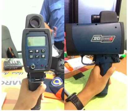
[image:5.612.316.530.109.252.2]

In the speed measurement calibration used a calibration tool in the form of speed gun owned by PT. Jasa Marga Persero (Tbk) Semarang Branch. The Speed Gun is derived from the speed calibration company called Laser Technology of the United States. Sightings of the speed gun, shown in Figure 4. Speed Gun is newly owned by PT. Jasa Marga Persero (PT) Semarang Branch in 2014, so that the written calibration date is March 23, 2014. The speed gun has a speed accuracy of ± 2 km/h

.

Figure 4: Speed Gun

4. System Evaluation Method

4.1. Vehicle Counting System

[image:5.612.91.297.387.567.2]

The evaluation measurements to calculate the number of vehicle is done by the method of prediction based data. Table 1 shows the conditions based on the comparison between the results of prediction systems with real conditions.

Table 1: Evaluation method based on test data and predictions (Powers, 2007)

Result of the comparison gives four possibilities, namely:

• True Positives (TP) = A vehicle is detected in

real conditions and declared as a vehicle on the systems.

• False Positives (FP) = None of vehicle is

detected in real conditions but declared as a vehicle on the systems.

• True Negatives (TN) = None of vehicle is

detected in real conditions and declared as not a vehicle on the systems.

• False Negative (FN) = A vehicle is detected in

real conditions but declared as not a vehicle on the systems.

Accuracy is the level of prediction that is closest to the actual label. Higher values of accuracy indicates better performance. The truth value of this parameter is calculated from the results of True Positive (TP) and True Negative (TN) divided by the combined results of the evaluation system consisting of True Positive (TP), True Negative (TN), False Positive (FP), and False Negative (FN). Evaluation for accuracy is represented by Formula 3.

(3)

4.2. Vehicle Speed Measurement System

In the vehicle speed measurement system, evaluation system is determined by analyzing the value of uncertainty which is obtained from the difference between the system’s speeds minus by the average difference, then divided by the amount of data retrieved, minus one. The formula to calculate the standard deviation is down below [8]:

Real Conditions

True False

System Results True TP FP

(6)

For:

= standar deviation

= Value of the difference between the measurement results and the speed gun = The average value of measurement result = Amount of data

After the standard deviation is obtained, it is then being followed by calculating measurement uncertainty. Measurement uncertainty is defined as a parameter associated with the measurement results which are expressed as a reasonable distribution of value that can be assigned to the measurand. If the estimated value of the measurand expressed by and the uncertainty of measurement, to a certain confidence level, expressed by , then the value of the measurand proficiency level is believed to be in the range according to the formula below:

(5)

In a measurement process, the uncertainty is estimated from observations of samples of the measurand ( ). Measuring the amount of n samples, standard uncertainty can be calculated using Equation 6 [9].

(6)

For:

= Uncertainty = Standard deviation = Amount of data

5. RESULT AND DISCUSSION

To determine the performance of the system made, testing needs to be done in order to take some of the original data in the form of video that records from the actual condition of the highway with the following specifications:

1. The duration of each video is ± 15 minutes. 2. The webcam has a frame rate of 30 fps. 3. The video resolution is 320 x 240 pixel.

4. The number of vehicles being shot by a speed gun should be at least 30 vehicles. This number is needed in order to analyze its uncertainty.

5.1. Testing In the Morning

[image:6.612.301.533.398.558.2]

It was still dark during the video taping, lux meter showed a value of 19 lux at an early time data retrieval and 118 lux at the end of data retrieval. Table 2 shows the calculation results of vehicle.

Table 2: Vehicles Calculation Results in the morning

No Conditions Amount Unit Total 1 The number of

passing vehicles in the real conditions

127 1 127

2 The number of vehicles counted in the systems

126

Counted as one 94 1 94

Counted as two 15 2 30

Distraction 2 1 2

Uncounted vehicles 18 1 18

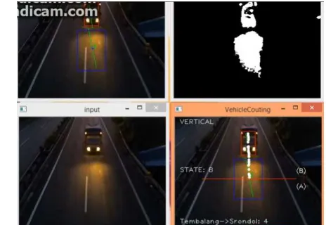
Sometimes one vehicle is detected as two due to the number of blob emergence. The cause of the emergence of more blob is due to the influence of spotlights from the vehicles. Spotlight vehicle is detected as a foreground, so that the system reads the spotlight as a blob. Figure 5 shows the creation of a vehicle that is counted as two vehicles.

Figure 5: A Vehicle is counted as two vehicles

The accuracy is obtained by using evaluation system based on data test.

(7)

ISSN: 1992-8645 www.jatit.org E-ISSN: 1817-3195 The results of vehicle’s speed measurement

results in the morning condition are presented in Table 3.

Table 3: Vehicle speed measurement results in the morning

Vehicle

Speed Program

(km/h)

Speed From

Speed gun

(km/h)

Difference (km/h)

Shooting Range

Speed gun (m)

1 88 51 -37 19.0

2 60 48 -12 25.3

3 62 57 -5 16.2

4 59 40 -19 34.3

5 90 63 -27 27.6

6 59 47 -12 24.2

7 60 46 -14 20.4

8 103 96 -7 27.3

9 61 78 17 23.4

10 59 54 -5 30.9

11 62 72 10 27.8

12 84 97 13 40.0

13 47 67 20 32.6

14 60 66 6 38.1

15 60 93 33 29.7

16 62 77 15 29.5

17 63 53 -10 23.3

18 66 74 8 30.8

19 60 65 5 25.2

20 47 58 11 27.7

21 59 72 13 29.8

22 62 66 4 31.2

23 60 86 26 39.1

24 61 72 11 21.2

25 92 42 -50 39.1

26 88 82 -6 28.6

27 89 72 -17 20.7

28 88 39 -49 29.5

29 58 90 32 39.4

30 61 77 16 45.2

31 59 26 -33 18.6

32 97 53 -44 19.1

33 58 79 21 18.8

34 61 98 37 34.3

35 113 92 -21 33.6

36 59 79 20 39.4

37 60 62 2 28.6

38 93 81 -12 23.8

39 60 56 -4 38.2

40 64 56 -8 40.8

41 88 80 -8 39.7

The number of vehicles that were shot by speed gun then being analyzed to obtain standard deviation and uncertainty value. Based on the analysis, the standard deviation obtained is 21.77 km/h. While the value obtained for the uncertainty is ± 3 km/h.

5.2 Testing In the Afternoon

[image:7.612.85.532.113.723.2]

Sufficient sunlight blazing includes data capture video during the afernoon, lux meter showed a value of 1598 lux at an early time data retrieval and 1922 lux at the end of data retrieval. Table 4 shows the calculation results of vehicle.

Table 4: Vehicles Calculation Results in the afternoon

No Conditions Amount Unit Total

1 The number of passing vehicles in the real conditions

155 1 155

146

During daylight condition, best value obtained is 90.5%. This is due to the absence of shadows that can cause noise in detecting the real number of vehicles. In this condition, it appears that the shadow falls just below the car and not widen.

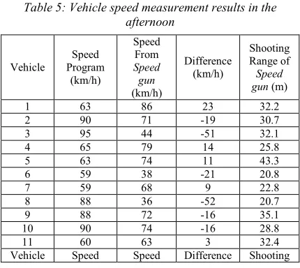
[image:7.612.310.525.546.738.2]

The results of vehicle’s speed measurement results during daylight condition are presented in Table 5.

Table 5: Vehicle speed measurement results in the afternoon

Vehicle

Speed Program

(km/h)

Speed From

Speed gun

(km/h)

Difference (km/h)

Shooting Range of

Speed gun (m)

1 63 86 23 32.2

2 90 71 -19 30.7

3 95 44 -51 32.1

4 65 79 14 25.8

5 63 74 11 43.3

6 59 38 -21 20.8

7 59 68 9 22.8

8 88 36 -52 20.7

9 88 72 -16 35.1

10 90 74 -16 28.8

11 60 63 3 32.4

(8)

ISSN: 1992-8645 www.jatit.org E-ISSN: 1817-3195 Program

(km/h)

From

Speed gun

(km/h)

(km/h) Range of

Speed gun (m)

12 60 66 6 35.9

13 88 40 -48 16.1

14 58 68 10 36.4

15 44 78 34 29.7

16 60 51 -9 22.2

17 60 89 29 24.6

18 92 57 -35 16.3

19 60 55 -5 19.2

20 59 91 32 23.7

21 90 59 -31 27.6

22 62 64 2 28.4

23 49 73 24 21.2

24 60 52 -8 20.0

25 60 54 -6 16.1

26 92 50 -42 37.1

27 60 80 20 27.9

28 64 107 43 27.8

29 62 73 11 31.5

30 60 70 10 35.2

31 61 80 19 38.6

32 62 61 -1 28.4

33 91 85 -6 45.3

34 60 86 26 42.0

35 101 70 -31 38.3

36 59 84 25 22.2

37 65 56 -9 29.3

38 59 89 30 27.1

39 60 56 -4 21.2

40 61 74 13 32.1

41 58 61 3 16.5

42 59 40 -19 35.3

43 91 75 -16 26.3

44 59 45 -14 26.1

45 58 54 -4 25.4

46 90 64 -26 32.0

47 89 79 -10 28.6

48 60 51 -9 29.4

49 63 81 18 33.2

50 61 60 -1 31.9

51 61 77 16 64.9

52 60 51 -9 40.8

The number of vehicles that were shot by speed gun then being analyzed to obtain standard deviation and uncertainty value. Based on the analysis, the standard deviation obtained is 22.90 km/h. While the value obtained for the uncertainty is ± 3 km/h.

5.3. Testing in the afternoon towards evening

Lux meter showed a value of 331 lux at an early time data retrieval and 0 lux at the end of data retrieval. Table 6 shows the results of the vehicle calculation in the afternoon towards evening.

Table 6: Vehicles Calculation Result in the afternoon towards evening

No Conditions Amount Unit Total 1 The number of

passing vehicles in the real conditions

240 1 240

227

Counted as three 3 3 9

The majority of errors are caused by a lot of uncounted vehicles, due to poor lightings conditions during the night. In the dark, the system could not distinguish between the background and the moving object (foreground). Moreover, tollways are not always equipped with adequate lightings.

[image:8.612.313.524.545.729.2]

The vehicle speed measurement’s results in the afternoon towards evening are presented in Table 7.

Table 7: Vehicle speed measurement results in the afternoon towards evening

Vehicle

Speed Program

(km/h)

Speed From

Speed gun

(km/h)

Difference (km/h)

Shooting Range of

Speed gun (m)

1 64 71 7 33.1

2 45 24 -21 16.9

3 60 76 16 34.7

4 67 93 26 27.9

5 61 71 10 24.9

6 59 120 61 32.4

7 59 71 12 23.4

8 66 65 -1 17.0

9 63 64 1 21.8

10 61 53 -8 41.6

11 92 61 -31 24.8

12 93 72 -21 26.9

13 63 67 4 40.8

(9)

Vehicle

Speed Program

(km/h)

Speed From

Speed gun

(km/h)

Difference (km/h)

Shooting Range of

Speed gun (m)

15 59 92 33 24.7

16 60 71 11 37.4

17 59 71 12 39.3

18 59 37 -22 28.0

19 59 44 -15 33.5

20 62 85 23 39.1

21 45 76 31 45.5

22 61 83 22 37.5

23 63 77 14 20.2

24 64 86 22 42.5

25 59 78 19 44.4

26 65 124 59 33.8

27 59 80 21 30.8

28 59 62 3 32.3

29 60 67 7 37.4

30 62 59 -3 31.3

31 58 56 -2 24.8

32 60 83 23 52.8

33 65 70 5 25.7

34 59 48 -11 24.4

35 59 65 6 36.6

36 63 81 18 19.2

37 61 55 -6 24.0

38 61 93 32 38.0

39 88 59 -29 40.0

40 62 62 0 27.0

41 61 72 11 29.7

42 59 48 -11 18.5

43 58 64 6 33.2

44 59 79 20 44.3

45 36 70 34 33.6

46 62 85 23 42.7

47 62 77 15 46.2

The number of vehicles that were shot by speed gun then being analyzed to obtain standard deviation and uncertainty value. Based on the analysis results, the standard deviation obtained is 19.55 km/h. While the value obtained for the uncertainty is ± 3 km/h

.

6. CONCLUSION & FUTURE WORKS

In this study, our systems can be used to count vehicle and its speed automatically in the highway. These systems have a better result in speed uncertainty because of the use of speed gun. These systems also have a good accuration in vehicle counting on three conditions namely in the morning, afternoon, and evening.

Based on the research results, the calculation process of the vehicle in the morning obtained 75.69 % in the accuracy value, while in the afternoon obtaining 90.50 %. Finally, in the evening, the accuracy value reached the percentage of 85.31 %. The measurement accuracy is also influenced by the shadow created below the vehicle

when passing on the highway. The uncertainty value for vehicle speed measurement is ± 3 km/h for all conditions.

To minimize the disruption in the form of shadow, a shadow remover program can be used or by enlarging the pixel size of the blob.

REFERENCES:

[1] AIPCR, Road Network Operations Handbook,

World Road Association, 2003.

[2] Thou-Ho Chen; Yu-Feng Lin; Tsong-Yi Chen, "Intelligent Vehicle Counting Method Based on Blob Analysis in Traffic Surveillance,"

Second International Conference on

Innovative Computing, Information and

Control, 5-7 Sept. 2007, pp.238-238

[3] Rahim, H.A.; Ahmad, R.B.; Zain, A.S.M.; Sheikh, U.U., "An adapted point based tracking for vehicle speed estimation in linear spacing," 2010 International Conferenece on Computer and Communication Engineering

(ICCCE), 11-12 May 2010 , pp.1-4.

[4] Nurhadiyatna, A.; Hardjono, B.; Wibisono, A.; Jatmiko, W.; Mursanto, P., "ITS information source: Vehicle speed measurement using camera as sensor," 2012 International Conference on Advanced Computer Science

and Information Systems (ICACSIS), 1-2 Dec.

2012, pp.179-184.

[5] Sina, I.; Wibisono, A.; Nurhadiyatna, A.; Hardjono, B.; Jatmiko, W.; Mursanto, P., "Vehicle counting and speed measurement using headlight detection," 2013 International Conference on Advanced Computer Science

and Information Systems (ICACSIS), 28-29

Sept. 2013, pp.149-154.

[6] Dehghani, A.; Pourmohammad, A., "Single camera vehicles speed measurement," 2013

8th Iranian Conference on Machine Vision

and Image Processing (MVIP), 10-12 Sept.

2013, pp.190-193.

[7] Powers, D.M.W., 2007. Evaluation: From Precison, Recall, and F-Factor to ROC,

Informedness, Markedness & Correlation,

Adelaide