APPLICATION OF SUPPORT VECTOR MACHINE IN LANE
CHANGE RECOGNITION
CHANG WANG,JIAHE QIN, REN ZHANG, YAQI ZHANG
School of Automobile, Chang’an University, Xi’an 710064, Shaanxi, China
ABSTRACT
Aiming at the lane change behavior recognition requirements for vehicle active safety system, natural driving test in real road were carried out and different parameters related to lane change behavior were collected synchronously. Firstly, parameters were processed with Kalman filter to increasing the potential relevance among sample data. Then, SVM model was established for lane change recognition. Lastly, data normalization, principal component analysis method, and bayesian network were adopted to optimize the SVM model. The recognize rate of lane change with 1.2 second time window increased from 93.9% to 98.7% by using these optimization measures. It can be meet the requirements of effectiveness and real-time for vehicle active safety system, such as lane change warning system or lane departure warning system.
Keywords: Lane Change, Support Vector, Kalman Filter, Principal Component Analysis, Bayesian
Network
1. INTRODUCTION
Lane change behavior was a general driving operation behavior, and it was also an important factor for driving safety. Accidents rate of lane change was higher than other conditions significantly. Statistic data shows that about 4% to 10% accident in Europe was caused by lane change [1]. Many researchers consider the lane change behavior was a difficult driving process for the drivers should pay more attention to the around traffic condition of subject vehicle, and the driving operation of steering wheel, accelerate pedal, and brake pedal were more frequent than other driving behavior [2]. Aiming at this problem, lane change warning system was proposed to assist drivers during lane change process. Generally, radars were adopted in lane change warning system in order to detect other vehicles around the subject vehicle. During the lane change process, if the radars detect other vehicles will be crashed with subject vehicle, the lane change system will alarming the driver to cancel lane change behavior [3]. So, it can be known that once the lane change warning system issued a warning signal, the system should confirmed that the subject vehicle had started the lane change process for avoiding false alarm. Therefore, how to recognize the starting of lane change was a key problem of lane change warning system.
Some algorithms were used for identification lane change behavior by using different parameters
of vehicle running state and driver’s operation behavior. Kristian Weiss and Nico Kaempchen used IMM(interacting multiple-model) algorithm to extend the single Kalman filter with the aim of improving tracking stability, and this model also be used to verify the effectiveness of lane change detect system [4]. Dongwook Kim Seungwuk Moon proposed a crash avoiding algorithm of ACC system. Emergency brake and lane change control algorithm were development considering the driving comfort, and longitudinal control and lateral control strategy were analyzed during the research process [5]. Hiren Mansukhlal Mandalia adopted HMM (Hidden Markov Model) and support vector method to recognize lane change intention, and the characterization parameters consisted of vehicle speed, steering angle, brake pedal position and distance between subject vehicle and front vehicles [6]. The verifying result showed that the support vector was most effective for the detecting of early stage of lane change behavior. Shigeki TEZUKA considers that driving behavior was consisted of several levels of status data, as driving awareness, driving skill and mental function [7].
steering angle were treated as characteristic parameters of lane change behavior recognize model above.
2. MODEL ESTABLISHMENT
2.1Support Vector Machine(SVM)
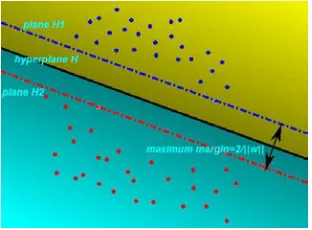
The direct target of using support vector was to classified characteristic data into several patterns. Generally, support vector can be divided into linear support vector and non-linear support vector according to the data dimension. Figure 1 is the classify principle of linear support vector, it can be seen that the plane H was a classify plane, but by rotating or translation the plane H, the new plane can also classified the data correctly. Although the classify plane was not uniquely, but the optimal hyperplane was exclusively. Optimal hyperplane was defined as the plane that had the biggest interval between plane H1 and H2.
Figure 1: Optimum Classify Plane For H1 And H2 Plane H in figure 1 was an optimal hyperplane, and plane H was parallel with plane H1 and H2. Optimal hyperplane H can be indicated as
( )
0
f x
= ⋅ + =
w x b
(1)Where w and x are n-dimension vector. For support vector model, X means input space and Y means output space. Component of X was treated as characteristic indicator. For dichotomous problem,
{ 1,1}
y= − . For multi-classification problems, the data format was:
(
) (
)
(
)
{
1, 1 , 2, 2 , , ,}
(
)
l l l
T= x y x y L x y ∈ ×x y
l is the sample number, xi represent the sample
and yi represent the label of lane change or lane
keeping. In this thesis, xi was a vector refers to the
lane markings distance and steering angle data of the sample data of i times. yi was the classification
[image:2.612.123.279.318.433.2]label with the value of 1 or -1. The value 1 represent the lane change behavior, and -1 represent the lane keeping behavior. The specific form was showed as follow.
Table 1: Data form supported of SVM Parameters Behavior label
-205, -200 4.463, 4.463 1 (lane change) -140, -140 4.463, 4.463 -1 (lane keeping)
-145, -150 8.925,8.925 -1 (lane keeping)
In general, multi-classification problem can be transformed to dichotomous classification in order to identification the specific pattern of the sample. For
{ }(
x y
i,
ii
=
1, 2, ,
L
l
)
, solving the minimalization of w for secondary fonctionelle as following [8]:2
1 min
2 w
The constraint condition was:
1 =1,2,
,
i i
y
⋅
w x
+ ≥ +
b
i
L
l
(2) For quadratic programming problem such as above, it can be transformed into the corresponding Lagrange dual problem for resolving. The Lagrange function of this problem is:(
)
2(
)
1 1
, , 1
2
l
i i i
i
L
α
w b wα
y w x b=
= −
∑
⋅ + − (3)i
α
is Lagrange multiplier andα ≥
i0
. According to Kuhn-Tucker condition, it can be get(
)
1
, , 0
l i i i i
L w b
w y x
w
α
α =
∂
= ⇒ =
∂
∑
(4)(
)
1
, ,
0
l i i i
L w b
y b
α
α = ∂
= =
∂
∑
(5)Substituted Equation 4 and Equation 5 into Equation 3, the dual optimization problem of original programming problem can be got as:
( )
1 1 1
1 max
2
l l l
i i j i j i j
i i j
L
α
α
α α
y y x x= = =
=
∑
−∑∑
⋅ (6)The corresponding constraint condition is
1
0,
0, =1,2,
,
l
i i i
i
y
α
α
i
l
=
=
≥
∑
L
(7)was imported, then, the original mapping problem can be transformed as:
1 1
{( , ), ( ,l l)}
T%= x y% L x y%
( )x%i =
φ
xi , and the classification plane is(
w x
% %
⋅ + =
)
b
%
0
, then2 , 1 1 min 2
. . (( ) ) 1) 1 , 1, ,
l
i w b
i
i i i
w C
s t y w x b i l
ξ ξ = + ⋅ + + ≥ − =
∑
% %% % L
(8)
The corresponding problem is [9]:
1 1 1
1
* *
1
* *
1
min ( , ) ,
2
. . 0
0
( , )
( ) sgn ( , )
l l l
i j i j i j j
i j j
l i i i
i
l
j i i i j i
i i i
y y K x x
s t y
C
b y y K x x
f x y K x x b
α α α α
α α α α = = = = = − = ≤ ≤ = − = +
∑∑
∑
∑
∑
∑
(9)The SVM in equation 9 is used widely, and it will be adopted for lane change behavior recognition in this paper.
2.2Characteristic Parameters
Parameters related to lane change behavior contains distance between vehicle and lane markings, steering angle, later accelerate, longitudinal accelerate, heading and others. Referring to the conclusion of other researchers and characteristic of parameters, feature set used in this paper contains two parameters as:
1. Distance d between subject vehicle and lane markings. The distance between subject vehicle and lane markings is the most directly characteristic parameter, and distance d can represent the lane change behavior quickly once the vehicle starts the lane change process.
2. Steering angle θ. Steering angle can represent the lane change process to a certain degree. For most lane change process, the steering angle will present a certain degree of changing, but the steering angle will be changed in other conditions except lane change. Therefore, by using steering angle unitarily, it can’t distinguish lane change behavior from curve road running of vehicle.
By using the feature set which contains distance d and steering angle θ, lane change behavior can be represented by this feature set comprehensively.
2.3Characteristic Parameters
Constrained by the measuring accuracy of sensors, the characteristic parameters contain some random errors, and the relevance among data will be reduced by this errors. The most important application of SVM was realized by excavation the potential relevance among characteristic parameters. So, in order to eliminate the random errors in original data, Kalman filter was adopted to dealing with the original parameters d and θ. Data gathered in natural driving test were discrete type in 10 Hz frequency, so discrete type Kalman filter was adopted. Setting the state variable of discrete
procedural is n
X∈R , and then the state equation and observation equation of discrete linear time-invariant system is
( )
(
1)
( )
( )
X k =AX k− +BU k +W k (10)
( )
( )
( )
Z k =HX k +V k (11)
W(k) and V(k) represent the incentive noise and observation noise, and there always be considered as white noise which complying with normality distribution independently.
( )
~(
0,)
p W N Q
( )
~(
0,)
p V N R
For calculation simplify, covariance matrix Q and R were supposed as constant.
( )
nX k R
− ∧
∈ (- means prior and ^ means estimate) is priori state estimate in step k based on the state before step k,
and
( )
nX k R
∧
∈ is posteriori state estimate of known measured variables Z(k) in step k. Then, the priori estimation error and posteriori estimation error can be defined as [10]:
( ) ( ) k
e X k X k
− ∧
−= − (12)
( )
( )
k
e X k X k ∧
= − (13)
The covariance of priori estimation error and posteriori estimation error is
( )
Tk k
P− k = E e e − − (14)
( )
Tk k
P k = E e e (15)
Priori estimation X
( )
k− ∧
can be revised by using observational variable and predictive variable as:
( )
( )
( )
( )
X k X k K Z k H X k
− −
∧ ∧ ∧
= + −
Difference between measure value and predicted value Z k
( )
−H X∧−( )
k
was referred to measure
residual, and it reflect the degree of agreement between predict value and actual value. Parameter K in equation 16 is residual gain, and it can be calculated as
(
)
TT T k
k k k T
k
P H
K P H HP H R
HP H R
−
− −
−
= + =
+ (17)
The function of k is to minimize the covariance of posteriori estimation error. With the increasing of gain parameter k, the weights of measure variable Z(k) will be increasing correspondingly, and this means the original gather data was more accurate. During the filter process, the state equation and observation equation can be written into
( )
( )
1 1
k k
k k
k k
s k
k k
S S
A Bu w
y k S
H v
yδ k
δ δ
δ − −
= + +
= +
(18)
,
k k
S
δ
were the original value of steering angle and distance of lane markings measured by sensors. W(k-1) and V(k) was white noisy with the mean value of 0.01. Initial value of X( )
0∧
is X(1), and P0 = 10, A = 1, B = 0. For the measured value was
came from original value, so H = 1. By using this Kalman filter model, parameter d and θ during lane change and lane keeping process will be filtered as following.
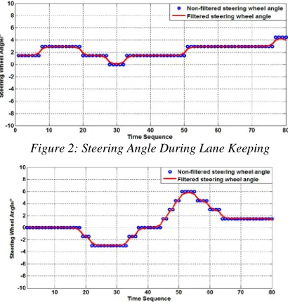
[image:4.612.312.522.74.344.2]Figure 2: Steering Angle During Lane Keeping
Figure 3: Steering Angle During Lane Change
Figure 4: Lane Markings Distance During Lane
Keeping
Figure 5: Lane Markings Distance During Lane Change
For original data, Kalman filter can improve the potential relevance and eliminate the random error in some degree. The filter result in figure above indicated that the original phase step type data were transformed into continuous smooth data, and the regularity of original data was enhanced significantly. Figure 3 shows that during lane change process, steering angle present sinusoidal variation approximately, and lane markings distance increased or decreased continuously. The difference between lane change and lane keeping was extended by using Kalman filter.
2.4Time Window Length
Time window length is an important factor for recognition rate of lane change behavior. If the time window length is too short, the lane change information contained in sample data will be insufficient and the recognition rate will be reduced. On the other hand, if the time window length is too long, the characteristic in feature set of lane change will be submerged by other disturb factors and the recognition rate will be reduced also.
Natural road lane change test result shows that the average lane change duration is 8.13s, and the average value time to line-crossing(TLC) is 2.33s. Therefore, when analyzing the length of suitable time window, it should comply with constricts as follow:
[image:4.612.93.298.503.718.2]traffic conflict was already existed for the subject vehicle had crossed the lane markings.
2. The SVM model should recognize the lane change behavior before the TLC moment. If the SVM model recognize the lane change behavior after the TLC moment, the traffic conflict will be existed before the TLC moment, ant this is not suitable for active safety system.
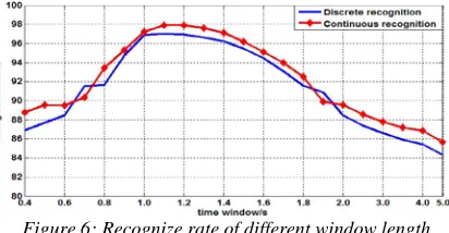
[image:5.612.96.302.249.356.2]According to constricts above, time length from 0.6 second to 5.0 seconds was used to test the recognize rate of lane change behavior in way of discrete value and continuous value.
Figure 6: Recognize rate of different window length Figure 6 shows that with the increasing of time window, the recognize rate increase from 85% to 94% about. But when the time window length achieved 1.2s, the recognize rate reduce from 97% to 85% when the time window achieved 5.0s. It can be known that the recognize rate of 1.2s is highest and it can achieve 94% approximately. Therefore, time window length 1.2s was used to carrying out lane change recognition.
2.5Data Normalization
During lane change process, the distance between vehicle and lane markings is in the range of -300 ~ +120 cm, while the range of steering wheel angle is typically less than 10°, so it existed large difference between the two parameters. The calculation will be more complex, and the time of training SVM will be longer for the large data range, which has negative impact on the SVM recognition accuracy. The data normalization method is usually used to reduce the complexity of data to reduce the amount of data calculation. The data normalized is carried out as:
(
max min) (
* min) (
/ max min)
miny= y −y x x− x −x +y (19)
Where ymax, ymin is the maximum and the
minimum value of y after normalized respectively, xmax and xmin are the maximum and minimum
values of the original data respectively. The steering wheel angle θ and the distance d between vehicle and lane markings can be normalized by using equation 19. An example is list as follow:
Original data: (2.975, 1.487, 0, -1.487, -2.975, 4.463, 7.438
)
TNormalized results: (0.1428, 0.1429, 0.4285, -0.7142, -1, 0.4285, 1
)
TOriginal data: (200, 195, 190, 185, 180, -175, -160
)
TNormalized results: (-1, -0.6667, -0.3333, 0, 0.3333, 0.6667, 1
)
T2.6Principal Component Analysis
For SVM model is suitable for binary classification problem, the multi-classification problem is usually transformed into binary classification problem, this means the high-dimensional data will be reduced into low-dimensional space by using the data low-dimensionality reduction method. Principal component analysis
(PCA) is a data dimensionality
reduction method with wide applications, and this method discards other non-primary factors by extracting the principal component of including feature information. In this way, we can
simplify the calculation
process, save the consumption resource during SVM running, and improve the speed of
training and testing. In
the actual application, the number of principal components is usually selected based on the
cumulative variance. In the premise of
ensuring accuracy, the fewer number of principal
components is, the more favorable for
the SVM model’s training and testing.
Suppose the research question contains p indicators, denoted as
1, 2 p
X X L X , which are the original variables. The principal component analysis is a linear combination
of these p indicators
to form new indicators
1, 2 p( )
F F L F k≤p according with the principle of retaining main information, fully reflecting the original variable information
and independence with each other.
The new variable expression is:
1 11 1 12 2 1
2 21 1 22 2 2
1 1 2 2
p p p p
k k k pk p
F u X u X u X F u X u X u X
F u X u X u X
= + + ⋅⋅⋅ +
= + + ⋅⋅⋅ +
⋅ ⋅ ⋅ ⋅ ⋅ ⋅
= + + ⋅⋅⋅ +
(20)
The general steps of principal component analysis are list as following:
Step 1: Solving the correlation
coefficient matrix
∑
X of the original variable.recognize involves 24 attribute variables, and the number of sample size is 1200. So the original sample matrix X can be expressed as
11 12 1,24
21 22 2,24
1200,1 1200,2 1200,24
x x x
x x x
X
x x x
= L L
M M M
L
(21)
Step 2: Solving the eigenvectors
and eigenvalues of the correlation matrix. 24
eigenvalues
λ λ
1≥ 2 ≥L ≥λ
24 and24 eigenvectors
1, 2 p
U U L U can be got by using
0
X
λ
I
∑ −
=
, where the eigenvector of the largest eigenvalue corresponds with coefficient vectorof the first principal component. The
eigenvector of larger eigenvalue corresponds with coefficient vector of the second principal component, and so on.
Step 3: Extracting the principal
component. Contribution rate is the proportion of the k principal component’s variance in the total variance. Cumulative contribution rate is the
proportion of the k principal
component’s variance in the total variance and it can describe the comprehensive ability of the first k principal components. The appropriate number of
principal components can be got
by calculating the contribution
rate of each principal component based on the contribution rate should larger or equal than 85%.
Based on the PCA method, lane change data and lane keeping data were processed, and the cumulative contribution rate is showed as
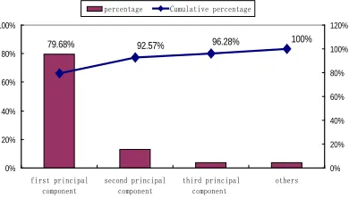
100% 96.28% 92.57% 79.68% 0% 20% 40% 60% 80% 100% first principal component second principal component third principal component others 0% 20% 40% 60% 80% 100% 120%
percentage Cumulative percentage
[image:6.612.334.521.135.260.2] [image:6.612.315.518.356.398.2]Figure 7: Cumulative Contribution Rate Distribution Figure 7 shows that the percent of first principal component and second principal component are larger, the amount percent of this two component achieved 92.57%. The third principal component account 3.71%, and the amount percent of all other components is 3.72%. This means the first principal component and second principal component occupy the main percent, so these two components are
adopted as the feature set. First principal component F1 and second principal F2 can be calculated as
1 2 3 4 5
6 7 8 9 10 1 11 12 13 14 15
16 17 18 19 20 21 22 23
0.885 0.916 0.885 0.916 0.924 0.938 0.948 0.959 0.964 0.965 0.960 0.958 0.954 0.948 0.930 0.925 0.894 0.846 0.822 0.803 0.766 0.738 0.766
X X X X X
X X X X X
F X X X X X
X X X X X
X X X
+ + + + +
+ + + + +
= + + + + +
+ + + + +
+ + 0.738X24
+ (22)
1 2 3 4 5 6 7 8 9 10 2 11 12 13 14 15
16 17 18 19 20 21 22
0.379 0.344 0.334 0.379 0.344 0.318 0.294 0.259 0.230 0.201 0.144 0.119 0.075 0.020 0.063 0.073 0.203 0.382 0.464 0.517 0.585 0.593 0.585
X X X X X
X X X X X
F X X X X X
X X X X X
X X
− − − − − +
− − − − − +
= − − − + + +
+ + + + +
+ + X23 0.593X24
+ (23)
2.7SVM Training and Testing
1200 times lane change data were gathered by natural driving test. The SVM training process used 900 sample data, and the other 300 data were used to test the SVM model. The training and test result were showed as following.
Table 2: Test result of SVM model Training Accuracy Testing Accuracy
1% FP 5% FP 1% FP 5% FP 63.26% 91.42% 73.14% 93.11%
The lane change behavior recognize result of SVM model can be represent by diagram as
[image:6.612.315.524.398.557.2]Figure 8: Result Of Lane Change Classification The curves in Figure 8 represent hyperplane, the area inside the curves referred to lane change, and the area outside the curves referred to lane keeping. The small circles in curves represent support vector. ‘+’ in figure 8 means lane change process was recognized into lane keeping process incorrectly. Correspondingly, and ‘*’ means lane keeping process was recognized into lane change behavior incorrectly. It can be seen from figure 8 that most lane change behavior was recognized correctly, but the result of SVM model not achieved 95%. In order to improve the recognize rate, the SVM model should be optimized in other ways.
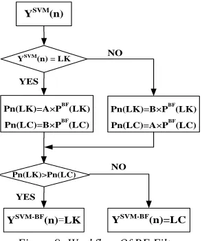
[image:6.612.102.297.514.625.2]In order to improve the recognize rate of lane change, bayesian network was introduced in this paper. Bayesian network is on the basis of SVM results. Bayesian filter(BF) takes fully the number of lane change and traffic environment into consideration and predicts driving behavior next moment. The predicted value and the actual output of SVM will be performed comprehensive analysis, and finally the recognition results of SVM-BF can be achieved [11]. This recognition process is shown in figure 9.
YSVM
(n)
Pn(LK)=A×PBF(LK)
Pn(LC)=B×PBF(LC)
YSVM
(n) = LK NO
YES
Pn(LK)=B×PBF(LK)
Pn(LC)=A×PBF(LC)
Pn(LK)>Pn(LC)
YES
NO
YSVM-BF(n)=LC
YSVM-BF
(n)=LK
[image:7.612.327.516.203.322.2]Figure 9: Workflow Of BF Filter
Where LK represent lane keeping and LC represent lane change. YSVM(n) is identification result of SVM at n moment. PBF(LK), PBF(LC) are respectively the probability of lane keep and lane change which are predicted by BF. Pn(LK), Pn(LC)
are respectively the corrected probability of lane keep and lane change. YSVM-BF(n) is identification result of SVM-BF model. According to equation as following, the model synthesizes SVM result and BF prediction result and gives the finally results of the model.
( )
( )
( )
' * y
* else
BF SVM
n n
n BF
n
A P LK if LK
P LK
B P LK
=
=
(24)
( )
( )
( )
' * y
* C else
BF SVM
n n
n BF
n
B P LC if LC P LC
A P L
=
=
(25)
( )
( )
' '
else
n n
SVM BF n
LK if P LK P LC y
LC
− = >
(26)
Where A and B were weight values. In order to ensure that the recognition results are genuine and believable, we take A and B as variable and they are determined by the range(Xmax-Xmin). The
maximum lane line distance ranges of lane keep are
statistically from 0 to 30 centimeters(considering the sampling precision of the instruments). The maximum ranges of lane change are 50.97 centimeters and its standard deviation is 35.58 centimeters. According to 3-σ criterion, the maximum lane line distance ranges in 1.2 second time window are from 0 to 160 centimeters. So, the abscissa of weights distribution curve is set between 0 and 160 centimeters.
Figure 10: Weights Distribution Curve Of A And B The expression of curve in this figure can be achieved by
( )
r s 0.2 0.8 0.036 sy ∆ = +s p qe∆ = + e− ∆ (27)
Through the verification, if the values of p, q and r are respectively 0.2, 0.8 and 0.036, the recognition rate of SVM-BF model is the highest one. If the output of the SVM is lane keeping, the value of A originates from the curve(shown above) and B is equal to one minus A. If the output of the SVM is lane change, the value of B originates from the curve(shown above) and A is equal to one minus B. Now we take 10 samples to explain the weights distribution process.
Table 3: Correction Of SVM Output Model type Output data
SVM recognition result -1, 1, -1, 1, -1 BF prediction value 0.37, 0.57, 0.39, 0.58, 0.40
SVM-BF output -1, 1, -1, 1, -1 actual result -1, 1, -1, 1, -1 SVM recognition result -1, -1, -1, -1, -1, BF prediction value 0.41, 0.61, 0.41, 0.61, 0.41
SVM-BF output -1, 1, -1, 1, -1 actual result -1, 1, -1, 1, -1
From table 3 we can see that the SVM outputs of the seventh and the ninth samples are lane keep and the probability of lane change which BF predicts exceed 0.5.That is to say that BF output and SVM output are inconsistent. In this case, the outputs of SVM and BF need to be comprehensive. Here the value of A and B are respectively 0.4 and 0.6.
( )
0.61 0.4( )
0.39 0.6 [image:7.612.128.275.238.413.2]Through calculation, the probability of lane change is greater than lane keep and SVM output will be corrected. The corrected result and actual result are consistent. It is obvious that BF can correct the false output of SVM to some extent and can improve the model recognition rate. In the test we collect 1200 samples and 900 samples are as the training sets and 300 samples are as the test sets. Finally, the recognition results of the model are listed as follow.
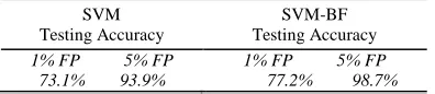
Table 4: Recognition Results Of SVM-BF Mode SVM
Testing Accuracy
SVM-BF Testing Accuracy 1% FP 5% FP 1% FP 5% FP
73.1% 93.9% 77.2% 98.7%
In general, the false positive rate accepted by engineering practice is 5%. Therefore, the contrastive analysis on the recognition rates of SVM and SVM-BF models is performed at 5% false positive rate. It is not difficult to see that SVM-BF recognition rate is nearly 5 percentages higher than SVM. Thus it can be seen that the generalization ability of SVM-BF model is stronger and its adaptability for samples is stronger. Recognize rate of 98.7% can satisfy the requirement of vehicle active safety system as lane change warning system, so the SVM model established by using the parameters of distance of lane markings and steering angle can be used in many fields, such as development process of vehicle safety systems, driving behavior researching and modeling, and so on.
4. CONCLUSION
Recognition of lane change behavior was important for the effectiveness of lane change warning system. Based on real road natural driving test, parameters related to lane change were gathered synchronously. Firstly, parameters were treated with Kalman filter to increasing the potential relevance between sample data. Then, SVM model was established for lane change recognizing. Lastly, data normalization, principal component analysis method, and bayesian network were adopted for optimize the SVM model. The recognize rate of lane change with 1.2s time window increased from 93.9% to 98.7% by using these optimization way. By using this SVM model, the instantaneity of vehicle active safety system can be improved significantly with high recognize rate, and the time reserved to drivers to avoid risk was more ample.
ACKNOWLEDGEMENTS
This work was supported by National Science Foundation of China under grant NO. 51178053 and supported by Program for Changjiang Scholars and Innovative Research Team in University under grant NO. IRT1286.
REFERENCES:
[1] Dario D Salvucci, Hiren M Mandalia, “Lane-change detection using a computational driver model”, Human Factors: The Journal of the Human Factors and Ergonomics Society, Vol. 49, No. 3, 2007, pp. 532-542.
[2] Weiss K, Kaempchen N, Kirchner A, “Multiple Model Tracking for the Detection of Lane Change Maneuvers”, IEEE Intelligent Vehicles Symposium, IEEE Conference Publishing Services, June 14-17, 2004, pp. 937~942.
[3] W Van Winsum, D De Waard, K A Brookhuis, “Lane Change Maneuvers and Safety Margins”, Transportation Research Part F, Vol. 2, No. 3, 1999, pp. 139-149.
[4] Rafael Toledo-Moreo, Zamora-Izquierdo M A,
“IMM-Based Lane-Change Prediction in
Highways with Low-Cost GPS/INS”, IEEE
Transactions on Intelligent Transportation Systems, Vol. 10, No. 1, 2009, pp. 180-185. [5] P A Barber, P King, M Richardson, “Road lane
trajectory estimation using yaw rate gyroscopes for intelligent vehicle control”, Transactions of the Institute of Measurement and Control, Vol. 20, No. 2, 1998, pp. 59-66.
[6] Hiren M Mandalia, Mandalia Dario D Salvucci, “Using Support Vector Machines for Lane-Change Detection”, Proceedings of the Human Factors and Ergonomics Society Annual Meeting, SAGE journals, September 2005, Vol. 49, No. 22, pp. 1965-1969.
[7] Tezuka S, Soma H, Tanifuji K, “A Study of Driver Behavior Inference Model at Time of Lane Change using Bayesian Networks”, IEEE
International Conference on Industrial
Technology, IEEE Conference Publishing Services, December 15-17, 2006, pp. 2308-2313.
behavior”, Transportation Research Part F, Vol. 5, No. 2, 2002, pp. 123-132.
[9] Michiel M Minderhoud, Piet H L Bovy, “Extended time-to-collision measures for road traffic safety assessment”, Accident Analysis and Prevention, Vol. 33, No. 1, 2001, pp. 89-97.
[10] R Toledo, M Zamora, B Ubeda, “High-integrity IMM EKF-based road vehicle navigation with low-cost GPS/SBAS/INS”, IEEE Trans. Intell. Transp. Syst., Vol. 8, No. 3, 2007, pp. 491-511. [11] Martijn Tideman, Mascha C, van der Voort, “A