Analysis of Internal Boundaries and Transition Regions in Geophysical Systems with Advanced Processing Techniques

(1)

Department of Physics and Astronomy, University of Canterbury,

Private Bag 4800, Christchurch 8140, New Zealand

Analysis of Internal Boundaries and

Transition Regions in Geophysical Systems

with Advanced Processing Techniques

A thesis

submitted in partial fulfilment

of the requirements for

a

Doctor of Philosophy in Physics

at the

University of Canterbury

by

Nikolai Christian Krützmann

University of Canterbury

2013

Supervisors: Dr. Adrian McDonald

Dr. Wolfgang Rack

(2)

(3)

Abstract

This thesis examines the utility of the Rényi entropy (RE), a measure of the complexity of probability density functions, as a tool for finding physically meaningful patterns in geophy-sical data. Initially, theREis applied to observational data of long-lived atmospheric tracers in order to analyse the dynamics of stratospheric transitions regions associated with barriers to horizontal mixing. Its wider applicability is investigated by testing the RE as a method for highlighting internal boundaries in snow and ice from ground penetrating radar (GPR) recordings. High-resolution 500 MHz GPR soundings of dry snow were acquired at several sites near Scott Base, Antarctica, in 2008 and 2009, with the aim of using the RE to facili-tate the identification and tracking of subsurface layers to extrapolate point measurements of accumulation from snow pits and firn cores to larger areas.

The atmospheric analysis focuses on applying the RE to observational tracer data from the EOS-MLS satellite instrument. Nitrous oxide (N2O) is shown to exhibit subtropicalRE

maxima in both hemispheres. These peaks are a measure of the tracer gradients that mark the transition between the tropics and the mid-latitudes in the stratosphere, also referred to as the edges of the tropical pipe. The RE maxima are shown to be located closer to the equator in winter than in summer. This agrees well with the expected behaviour of the tropical pipe edges and is similar to results reported by other studies. Compared to other stratospheric mixing metrics, theREhas the advantage that it is easy to calculate as it does not, for example, require conversion to equivalent latitude and does not rely on dynamical information such as wind fields.

The RE analysis also reveals occasional sudden poleward shifts of the southern hemis-phere tropical pipe edge during austral winter which are accompanied by increased mid-latitude N2O levels. These events are investigated in more detail by creating daily

high-resolution N2O maps using a two-dimensional trajectory model and MERRA reanalysis

winds to advect N2O observations forwards and backwards in time on isentropic surfaces.

With the aid of this ‘domain filling’ technique it is illustrated that the increase in southern hemisphere mid-latitude N2O during austral winter is probably the result of the cumulative

effect of several large-scale, episodic leaks of N2O-rich air from the tropical pipe. A

com-parison with the global distribution of potential vorticity strongly suggests that irreversible mixing related to planetary wave breaking is the cause of the leak events. Between 2004 and 2011 the large-scale leaks are shown to occur approximately every second year and a connec-tion to the equatorial quasi-biennial oscillaconnec-tion is found to be likely, though this cannot be established conclusively due to the relatively short data set.

Identification and tracking of subsurface boundaries, such as ice layers in snow or the bedrock of a glacier, is the focus of the cryospheric part of this project. The utility of theRE

(4)

a similar (high) value, resulting in a clear contrast between reflections and background scattering. Additionally, theoretical considerations allow the definition of a ‘standard’ data window size with which the RE can be applied to recordings made by most pulsed GPR systems and centre frequencies. This is confirmed by tests with higher frequency recordings (50 and 500 MHz) acquired on the McMurdo Ice Shelf. However, these also reveal that the

RE processing is less reliable for identifying more closely spaced reflections from internal layers in dry snow.

(5)

Acknowledgements

First of all, I would like to thank my supervisors Adrian McDonald, Wolfgang Rack, and Steve George for allowing me to undertake this somewhat unconventional project. It has been a pleasure working with all three of you and I greatly appreciate your constant readiness to provide advice, knowledge, or copious amounts of feedback when required, as well as guidance and encouragement, particularly when things were not going so well. Without your continued support, this work and especially its completion would not have been possible.

I also want to thank my long- and short-term office mates: Mita Brierly, Simon Parsons, Jack Coggins, Robert Ward, Madeleine Smith, and Jakob Grahn for their great company, helpful advice, and fun chats that kept me socialised during the more intensive periods of this research, and for not minding to work in an office that is occasionally misused as a bedroom. Thank you also to Karl Howley and Phillippa Dobson for putting up with a flat mate who has never heard of keeping regular hours and starts to bake bread at 2:00 am, and for generally being the best flat mates I could have wished for. Special thanks go to Mette Riger-Kusk for her participation in the Antarctic field work in 2008, her amazing skills with duct tape, and also for the radar data from the Touchdown Glacier (Antarctica) that is used in this thesis.

I am also very grateful to all the institutions who have provided me with financial support along the way, such as the University of Canterbury, the UC Department of Physics & Astronomy, and Gateway Antarctica. The support of the Antarctic measurement campaigns from the Christchurch City Council and by Antarctica New Zealand under the field event K053 ‘Cryosphere Remote Sensing’ is greatly appreciated. Furthermore, I want to thank Nick Key and Justin Harrison from the UC Department of Geography who were of great assistance during the preparations for the field campaigns, the Scott Base staff for great support and an enjoyable time in Antarctica, and Bob Noonan for assisting with some of the preparation and processing of the radar data.

(6)

1 Introduction 1

1.1 Motivation . . . 1

1.2 Thesis Outline . . . 3

2 Geophysical Background 5 2.1 Atmospheric Structure and Stratospheric Dynamics . . . 5

2.1.1 Stratospheric Tracers . . . 11

2.1.2 Isentropic Potential Vorticity . . . 14

2.1.3 The Equatorial Quasi-Biennial Oscillation . . . 15

2.2 Tracer Data Processing with Rényi Entropy (RE) . . . 19

2.3 Atmospheric Data Sets . . . 22

2.3.1 SOCOL Chemistry-Climate Model . . . 23

2.3.2 MERRA Reanalysis . . . 23

2.3.3 EOS-MLS Observations . . . 24

2.3.3.1 Nitrous Oxide . . . 27

2.3.3.2 Methyl Chloride . . . 27

2.3.3.3 Carbon Monoxide . . . 29

2.3.4 Trajectory Model . . . 30

2.4 Ground Penetrating Radar in Cryospheric Studies . . . 32

2.4.1 Accumulation and Compaction of Snow . . . 33

2.4.2 Dielectric Properties of Snow and Ice . . . 35

2.5 Conventional GPR Processing . . . 36

2.5.1 Nonstationarity Correction (Dewow) . . . 36

2.5.2 Range Power Loss Compensation (Gain) . . . 38

2.5.3 Frequency Filters . . . 39

2.5.4 Stacking and Background Subtraction . . . 39

2.5.5 Envelope Calculation . . . 40

2.6 Cryospheric Data Acquisition . . . 42

2.6.1 Stake farms, Snow Pits, and Firn Cores . . . 42

(7)

List of Figures

2.1 The lower layers of the atmosphere . . . 6

2.2 Altitude, pressure, and potential temperature levels for October 2009. . . 8

2.3 Meridional structure of the stratosphere . . . 9

2.4 Trace gas residence times and associated mixing scales . . . 12

2.5 Average zonal mean nitrous oxide (N2O) for October from 2004 to 2011 . . . 13

2.6 Zonal mean zonal winds at the equator from August 2004 through April 2011 16 2.7 Illustration of the mechanism of the QBO . . . 17

2.8 The Holton-Tan effect . . . 18

2.9 Meridional profile of the REz10 and underlying histograms. . . 21

2.10 Zonal mean nitrous oxide (N2O) at 850 K and 550 K . . . 26

2.11 Zonal mean methyl chloride (CH3Cl) at 550 K . . . 28

2.12 Zonal mean carbon monoxide (CO) at 850 K . . . 29

2.13 Comparison of 2D trajectory model and HYSPLIT trajectories . . . 31

2.14 Effect of dewow and running mean filters on a 500 MHz trace . . . 37

2.15 Location of the Antarctic measurement sites . . . 43

2.16 Snow pit and dust layer (2008) . . . 44

2.17 Coring setup and firn core (2009) . . . 45

2.18 500 MHz and 1 GHz GPR setup and data acquisition . . . 47

2.19 50 MHz GPR setup . . . 48

2.20 The Darwin-Hatherton glacial system . . . 50

3.1 Global versus optimal binning with SOCOL data . . . 54

3.2 REz10 of EOS-MLS N2O data at 850K for 2008 . . . 55

3.3 REz10 of N2O and CH3Cl at 550K for 2008 . . . 56

3.4 REz10 of N2O with added noise and REz10la3 of CH3Cl at 550K for 2008 . 58 3.5 REz10 of CO data at 850K for 2008 . . . 59

3.6 Climatology ofREz10 at 850 K derived from MLS N2O data from 2004 to 2011 61 3.7 Subtropical peak ofREz10 at 850K from August 2004 to December 2005 . . 65

3.8 Zonal mean zonal winds andN2O at 850 K in the southern hemisphere . . . 67

(10)

3.10 Meridional profile of monthly meanREz10 for August 2005 . . . 70

3.11 Evolution of the tropical pipe edge at 550K and 850 K. . . . 72

3.12 Evolution of zonal mean N2O at 36°S in 2005, 2008, and 2010 . . . 73

3.13 Evolution of zonal mean N2O at 21°S, 36°S, 51°S, and 60°S in 2009 . . . 74

3.14 Vertical profile of monthly meanREz10 for July of 2006, 2008, 2009, and 2010 77 3.15 Domain filled map ofN2O at 850 K for 28.6.2009 . . . 80

3.16 Domain filled map ofN2O at 850 K for 19.8.2009 . . . 81

3.18 Domain filled maps for leak event in July 2009 . . . 83

3.20 RMSD ofN2O at 850 K . . . 86

3.22 Zonal mean N2O at 51°S vs. RMSD in 2009 at 850 K . . . 88

3.23 RE for domain filled maps at 850 K for selected days . . . 90

3.24 Polar plot of QBO phase vs.N2O at 850 K . . . 94

3.25 Amplitudes of waves 1, 2, and 3 at 850K in 2008 . . . 97

3.26 A zonally symmetric tracer gradient and its REla5 . . . 97

3.27 A weakly distorted tracer gradient and itsREla5 . . . 98

3.28 A strongly distorted tracer gradient and itsREla5 . . . 98

3.29 A stronlgy distorted tracer gradient with offset and its REla5 . . . 99

4.1 Synthetic gradient test of RE . . . 103

4.2 Synthetic gradient test of RE with increased noise level . . . 103

4.3 RE25h8v of raw 25 MHz data . . . 105

4.4 RE25h8v of dewowed and enveloped data. . . 106

4.5 RE25h8v after three outlier removal iterations . . . 107

4.6 RE25h8v after five and ten outlier removal iterations . . . 108

4.7 Remaining data points after one, three, five, and ten iterations . . . 110

4.8 RE derived from larger histograms . . . 112

4.9 Number of bins selected by optBINS . . . 113

4.10 RE25h8v calculated with ten and thirty fixed bins . . . 114

4.11 RE25h8v using α= 1 and α= 5. . . 116

4.12 Radargram with regular processing . . . 118

4.13 Comparison of basic gaining andRE20h10v-results for a 25MHz profile . . . . 119

4.14 RE20h10v of a 50 MHz profile . . . 121

4.15 Comparison of RE20h10v applied to 50 and 500 MHz data . . . 123

(11)

List of Figures

5.1 Blackman-Harris pulse and its spectrum . . . 132

5.2 Dielectric model for GPR simulation . . . 134

5.3 Simulated GPR trace and profile . . . 135

5.4 Envelope of simple simulated GPR profile . . . 136

5.5 Layer thickness estimated from simulated radargram . . . 137

5.6 Average simulated ground-reflection and its spectrum . . . 137

5.7 Simulated trace and its spectrum after deconvolution without a low-pass . . 138

5.8 Simulated trace after deconvolution and 1100MHz low-pass filtering . . . 139

5.9 Deconvolved GPR profile including a 1100MHz low-pass . . . 140

5.10 Layer depth and thickness from deconvolved GPR profile . . . 140

5.11 Simulated GPR profile with added noise and derived layer thickness . . . 141

5.12 Deconvolved GPR profile with added noise and derived layer thickness . . . 142

5.13 Emitted signal and frequency spectrum of the 500 MHz GPR system . . . . 144

5.14 The effect of standard processing and deconvolution on a GPR profile from L2 146 5.15 Spectrum and autocorrelation of a trace before and after deconvolution . . . 147

5.16 Trace and envelope of a reflection before and after deconvolution . . . 148

5.17 A deep reflection at L2 and its spectrum . . . 149

5.18 Snow density profiles from L2 and L3 for 2009 . . . 151

5.19 Processed radargrams and tracked layers at L2 for 2008 and 2009 . . . 153

5.20 Interpolated accumulation maps for L2 and L3 . . . 154

5.21 Processed radargram of L3 from 2009 . . . 155

5.22 Accumulation along a transect from L2 to L1 . . . 157

5.23 Snow compaction derived from repeat GPR measurements at L2 . . . 158

(12)

2.1 EOS-MLS data characteristics . . . 25

5.1 Summary of accumulation measurements . . . 152

(13)

Abbreviations

CH3Cl Methyl chloride

CH4 Methane

CO Carbon monoxide

N2O Nitrous oxide

ACF Autocorrelation function

AGC Automatic gain control

BDC Brewer-Dobson Circulation

DFT Discrete Fourier transform

DJF December, January, February

DVL Data video logger (pulse EKKO PRO)

EOS Earth Observing Systems

FDTD Finite-difference time-domain (model)

FFT Fast Fourier transform

FT Fourier transform

GMT Greewich Mean Time

GPR Ground penetrating radar

GPS Global Positioning System

HT Hilbert transform

HYSPLIT Hybrid Single Particle Lagrangian Integrated Trajectory Model

IFT Inverse Fourier transform

iHT Inverse Hilbert transform

(14)

MAM March, April, May

MERRA Modern Era Retrospective analysis for Research and Applications

MLS Microwave limb sounder

NCAR National Center for Atmospheric Research

NCEP National Centers for Environmental Prediction

PDF Probability distribution function

ppbv Parts per billion by volume

pptv Parts per trillion by volume

PV Potential vorticity

PVU potential vorticity unit (1·10−6 m2_K

s·kg )

QBO Quasi-biennial oscillation

RE Rényi entropy

RMSD Root mean square deviation

SEC Spreading and exponential compensation

SOCOL SOlar Climate Ozone Links (chemistry-climate model)

SON September, October, November

TWT Two-way-travel time

UTC Coordinated Universal Time, same as GMT

(15)

Chapter 1 Introduction

1.1 Motivation

Most real world geophysical systems are complex, meaning they are non-linear and often dis-play irregular patterns as a result of the interactions and interdependencies of the numerous physical processes involved in the system. Measures of complexity are a means of analysing such intricate systems. Similar to statistical methods, they are a way of “standing back” and investigating the behaviour of the system as a whole, instead of trying to understand and model all its details with perfect accuracy. By identifying regions where transitions occur, complexity measures can highlight key areas of a geophysical system, thereby giving detailed information about a complex system in a simple way.

The Rényi entropy (RE) is a statistical complexity measure that was established as an efficient tool for identifying tracer gradients associated with stratospheric barriers to horizontal mixing in Krützmann et al. (2008) and Krützmann (2008). Having successfully applied this measure to tracer data from climate model simulations, one objective of this thesis is to use theREto study the properties and behaviour of stratospheric mixing barriers in more detail by applying it to satellite observations. Being a statistical measure based on (discrete) probability density functions (PDFs), the RE can be calculated for any kind of numerical data set. Therefore, the second objective is to investigate the applicability of the RE methodology to other geophysical systems. In particular, the RE’s utility for detecting amplitude gradients in cryospheric ground penetrating radar (GPR) measurements is examined. To this end, high-frequency GPR profiles of dry snow were recorded at several locations in the vicinity of Scott Base on Ross Island, Antarctica. Identifying and tracking internal layers in this data, in order to extrapolate point measurements of accumulation from snow pits and firn cores to larger areas, is the third objective of the present work.

(16)

the main source for many stratospheric trace gases, it constitutes one of the most important links between the troposphere and the stratosphere. Neu et al. (2003) and more recently

Palazzi et al. (2011) investigated the dynamics of these mixing barriers, yet they are still far from being fully understood. A detailed analysis of the (sub-)tropical mixing barriers is performed in the present work by applying theRE to stratospheric tracer observations from the Earth Observing System Microwave Limb Sounder (EOS-MLS) satellite instrument, in order to improve the understanding of the evolution of the tropical pipe.

Being fundamentally sensitive to gradients, theREcan potentially also detect transition regions in other geophysical data sets. In snow and ice, transition regions are associated with boundaries between internal layers created by changes in the ambient conditions at the time of deposition. By identifying and tracing internal layers using high-frequency, pulsed GPR measurements of the Antarctic snow cover, changes in the depth and spacing of the layers in snow can be used to determine accumulation and compaction over time (e.g. Arcone et al., 2005). This information is important for validation of satellite altimeter observations used for estimating the polar mass balance, since snow accumulation and snow compaction need to be separated in order to quantify imbalances from satellite derived surface elevation change (Wingham et al., 2006). Similarly, low-frequency GPR profiles can be used to determine the subsurface topography and thickness of Antarctic glaciers (e.g. Bogorodsky et al., 1985), information which is also very important for mass balance calculations. In both cases, the contrast between layers with different dielectric properties, e.g. dense snow vs. depth hoar or ice vs. subglacial rock, causes partial reflection of the GPR pulse and thereby a change in received signal amplitude. These amplitude gradients can potentially be detected with the

RE, similar to the detection of tracer gradients in the stratosphere.

The intensity of the signal recorded with GPR soundings can vary over several orders of magnitude. Accordingly, a considerable number of processing steps are often required to allow identification of subsurface structures. The RE, being a relative measure, is independent of the absolute values in a data set and can therefore potentially detect amplitude gradients of varying intensity without requiring additional processing. In an atmospheric context, the

RE has also been shown to be more efficient when analysing large amounts of data than other, more elaborate processing techniques (Krützmann, 2008). This can be advantageous when considering initial data processing of GPR recordings in the field, where the available time and computational power is often limited. Additionally, the statistical nature of theRE

entails that, while numerous data points are required to calculate one RE value, individual outliers or data gaps caused for example, by disturbances of the measuring equipment, can be excluded to improve the results.

(17)

1.2. Thesis Outline

1.2 Thesis Outline

This thesis is structured into four main chapters and a final chapter that summarises the results. Chapter 2 introduces the geophysical background material and is split into two parts. The first half starts with an overview of the structure of the atmosphere and the stratosphere in particular, followed by explanations of several relevant concepts, such as potential vorticity (PV), the quasi-biennial oscillation (QBO), and the use of long-lived chemical tracers for understanding stratospheric dynamics. Next, a methodology for using the RE to detect mixing barriers in measurements of stratospheric tracer concentrations is introduced. Details are then given regarding the data sets that are used for the atmospheric analyses in Ch. 3, such as the tracer observations from the EOS-MLS satellite instrument and the MERRA reanalysis data. In the second half of Ch. 2 an overview of the applications of GPR for studies of the cryosphere is given and the relevant dielectric properties of snow and ice are discussed. This is followed by a summary of several processing steps often applied to GPR data. Finally, the location and setup of the measurement campaign in Antarctica is described, the methodologies used for data acquisition are introduced, and the setup and specifications of the GPR equipment are detailed. Additionally, the origin of a 25MHz GPR cross-section of an Antarctic glacier used in Ch. 4 is briefly explained.

Chapter 3 begins with the introduction of a ‘global binning’ method for atmospheric tracer data that is different from the previously used ‘optimal binning’ procedure for creating the PDFs from which the RE is calculated, and its advantages are highlighted. The new approach is applied to EOS-MLS observations of several stratospheric trace gases: nitrous oxide (N2O), methyl chloride (CH3Cl), and carbon monoxide (CO). Comparison of the

results leads to insights about the effects of noise on theREpatterns and the comparability of different trace species. Additionally, a seven-year climatology of theREofN2O observations

is presented, followed by a detailed analysis of the evolution of the mixing barriers at the edges of the tropical pipe in the lower and middle stratosphere as identified by the RE of

N2O between 2004 and 2011. The results are compared with previous work and lead to the

detection of several periods during which considerable amounts of N2O-rich air appear to

‘leak’ from the tropics into the southern hemisphere surf-zone during austral winter. The temporal evolution and vertical extent of these ‘leak events’ is then investigated and changes in the vertical structure of the tropical pipe when these leaks occur are discussed. The dynamics leading to the tropical leaks are examined by using ‘domain filling’, a method for artificially enhancing the number of N2O observations for a particular day by using a

trajectory model. The applicability of the RE to the high-resolution domain filled maps for investigating longitudinal variability of the tropical pipe edges is also investigated. Finally, the results are summarised and a potential link between the occurrence of tropical leaks and the phase of the QBO is discussed.

Before applying the RE to cryospheric GPR observations, a sensitivity study of the

(18)

of varying parameters such as the data window size, the number of bins for the histograms, or the exponent of the RE are tested. The RE patterns are then compared to the results of a more conventional processing methodology and differences are discussed. This leads to guidelines for applying the RE to a wider variety of GPR recordings, which are tested on higher frequency (50 and 500 MHz) profiles of the McMurdo Ice Shelf (Antarctica) in the last part of the chapter. The results are then summarised and conclusions regarding the utility of the RE as an alternative pseudo gain function for initial analysis of GPR data in the field are drawn.

Due to some limitations of the RE methodology when it comes to identifying multiple closely spaced gradients, the RE is not ideal for identifying and tracking relatively weak reflections related to internal layers in dry snow. Consequently, an alternative processing approach, the deterministic Fourier deconvolution is developed in Ch. 5, which is particu-larly suitable for GPR recordings of relatively low-contrast media. The deterministic Fourier deconvolution is first tested on a simulated radar profile and then applied to 500M Hz GPR data of dry polar snow. The established stake farms as well as information on snow density and internal layering from snow pits and firn cores are used to estimate accumulation rates over several years at the measurements sites. By identifying and tracking internal layers in the deconvolved GPR profiles, the accumulation estimates are then expanded to larger areas. Furthermore, the change in the separation of individual reflection horizons from one year to the next is used to calculate snow compaction rates down to 13 m depth. The derived accumulation and compaction rates are compared to previous studies and differences are discussed, before giving a summary of the results and drawing conclusions regarding the wider applicability of the presented processing technique.

Chapter 6 summarises the findings of the previous chapters and outlines future work that could be pursued as a result of these.

Additionally, this thesis has an electronic supplement containing several animations of domain filled maps of N2O. The filenames and some details about the individual animations

(19)

Chapter 2 Geophysical Background

Some parts of this chapter are derived from the article “Snow accumulation and compaction derived from GPR data near Ross Island, Antarctica” published in the online journal The Cryosphere (Kruetzmann et al., 2011).

This chapter introduces the atmospheric and cryospheric context for the work presented in the following chapters and illustrates a number of basic concepts from the two fields. Additionally, details are given about the different data sets that will be used.

Section 2.1 gives an overview of the atmospheric structure and the stratosphere in par-ticular. The role of chemical tracers in the stratosphere and how these can be used to gain information about stratospheric dynamics is discussed, followed by an explanation of poten-tial vorticity and the quasi-biennial oscillation. Section 2.2 describes how the Rényi entropy (RE) statistical measure can identify tracer gradients associated with mixing barriers in stratospheric tracer data. In Sect. 2.3, various data sets used for the atmosphere-related part of this thesis (Ch. 3) are introduced. The second half of this chapter begins with an over-view of the utility of ground penetrating radar (GPR) for glaciological studies and for the detection of internal layers in particular (Sect. 2.4), followed by a discussion of the dielectric properties of snow and ice. Section 2.5 then introduces a number of basic processing steps commonly applied to GPR recordings. Section 2.6 illustrates the location and layout of the sites of the Antarctic measurement campaign and explains how the snow accumulation and density information used in Ch. 5 was acquired from stake farms, snow pits, and firn cores. Furthermore, the specifications of the GPR system are given and the different setups used for 50 and 500 MHz data acquisition are described. Additionally, the origin and acquisition parameters of a 25 MHz GPR cross-section of a glacier in the Trans-Antarctic Mountains, analysed in Ch. 4, is detailed.

2.1 Atmospheric Structure and Stratospheric

Dyna-mics

(20)

refer-Figure 2.1: The lowest three layers of the atmosphere and the evolution of the (mean) temperature with altitude. The boundaries between layers are characterised by a reversal of the temperature gradient (from Andrews, 2000).

red to as the “pauses”, i.e. the tropopause, the stratopause, etc. This structure is illustrated in Fig. 2.1 for the three layers closest to the surface.

Figure 2.1 also shows that both height (above sea level) and pressure can be used as a vertical coordinate. The approximate altitude, z, of a particular pressure level, p, can be calculated by:

z(p) = R·T

g ·ln po

p

!

(2.1)

where R ≈287.05 J

kg K is the specific gas constant for dry air, p0 ≈1013hPa is the average

pressure at sea level, T = 255K is the approximate average temperature of the troposphere and stratosphere (Wallace and Hobbs, 2006), andg _≈9.8m_s2 is the acceleration due to gravity, taken to be constant in this case. Equation 2.1 can be derived from the hydrostatic equation:

∂p

∂z =−g·ρ (2.2)

whereρis the density of air, which assumes that the air is in hydrostatic equilibrium, meaning that the pressure at a particular point is determined only by the mass per unit area of the column of air above that point. Using the ideal gas law in its molar form (with R being the specific gas constant for dry air as above):

p=ρRT (2.3)

ρ can be eliminated from Eq. 2.2. Rearranging and integrating from the surface (z = 0,

p=p0) to altitudez and pressurep, assuming an isothermal atmosphere with a temperature

[image:20.595.158.387.62.286.2]

(21)

2.1. Atmospheric Structure and Stratospheric Dynamics

The troposphere is the layer closest to the Earth’s surface and is therefore also the region in which “weather” occurs. It is associated with turbulent dynamics and strong vertical and horizontal mixing as the negative temperature gradient (or lapse rate) with altitude makes the troposphere inherently unstable (Andrews, 2000). Additionally, the Earth’s surface absorbs large amounts of solar radiation which in turn heats up the air close to the surface. This results in strong convective mixing processes, particularly at the equator, and causes the air in the troposphere to be relatively well mixed in the vertical. The transition region above the troposphere, the tropopause, can be defined as “the lowest level at which the lapse rate decreases to 2˚C

km or less, provided that the average lapse rate between this level and all

higher levels within 2km does not exceed 2 ˚C

km.” (World Meteorological Organization, 1992)

The tropopause isolates the troposphere from the stratosphere, as it only allows limited transport between these regions, and its height tends to decrease with latitude (Shepherd, 2003).

As the name suggests, the stratosphere is highly stratified in most cases and vertical trans-port and mixing is limited (Wallace and Hobbs, 2006). The positive temperature gradient in the stratosphere implies that the region is much more stable with regards to convective mixing than the troposphere. Combined with the fact that it is close to radiative equili-brium (Shepherd, 2003), this results in the stratosphere being stably stratified on potential temperature surfaces. The potential temperature, θ, for an ideal gas at pressure, p, can be calculated as:

θ =T · p0

p

!_cpR

(2.4)

where p0 is the surface pressure (often taken as 1000 hPa everywhere for simplicity), cp ≈

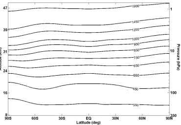
1.003_{kg K}kJ is the specific heat capacity of air at constant pressure, andT is the temperature of the air in K.The potential temperature of a volume of air (or air parcel) corresponds to the temperature the air would have if it were compressed until it reaches the (assumed) surface pressure, without adding or removing heat, i.e. adiabatically (Wallace and Hobbs, 2006). As the stratosphere is approximately in radiative equilibrium, the heat required for diabatic changes to an air parcel is not readily available, which is why short-term motions (5-10 days) largely occur on potential temperature surfaces (Holton et al., 1995). Therefore, potential temperature is often used as an alternative vertical coordinate to altitude or pressure in studies of the stratosphere. It is particularly useful when the short-term motion of individual air parcels is being considered, since the three-dimensional problem can be reduced to two-dimensional motion on a potential temperature surface by ignoring the (weak) diabatic effects. Figure 2.2 shows the zonal average altitude and pressure of a number of potential temperature levels derived from the monthly zonal1 mean temperature data for October 2009 (MERRA reanalysis, see also Sect. 2.3.2), illustrating the approximately horizontal nature of potential temperature surfaces. Note that the altitude scale in Fig. 2.2 is derived from an exponential fit to the tabulated values of the U.S. Standard Atmosphere 1976 (U.S. Government Printing Office, 1976), which results in a slightly lower altitude for each pressure level than the use of Eq. 2.1.

(22)

Figure 2.2: Relationship between altitude, pressure, and potential temperature contours (in

K) in the stratosphere, derived from monthly zonal mean MERRA temperature data for October 2009.

Figure 2.2 also illustrates that the potential temperature increases with altitude, i.e. that

∂θ

∂z > 0 throughout the stratosphere. This is important with respect to the stability of the

stratosphere: it can be shown that the behaviour of an air parcel that has been displaced adiabatically in the vertical is directly related to the local gradient in potential temperature. If the gradient is positive (∂θ

∂z >0), the air parcel will rebound and begin to oscillate around

its equilibrium position with the Brunt-Väisälä frequency (Wallace and Hobbs, 2006):

N =

s

g θ ·

∂θ

∂z (2.5)

Barring any other external forces, the oscillation will be gradually damped by viscous forces, eventually returning the air parcel to its original altitude. If on the other hand, the poten-tial temperature gradient is negative (∂θ_∂z < 0), Eq. 2.5 gives an imaginary Brunt-Väisälä frequency which means that the air parcel will not begin to oscillate but continue to move away from its original position (Wallace and Hobbs, 2006). Accordingly, the atmosphere is statically stable when ∂θ_∂z >0, and statically unstable if ∂θ_∂z <0.

[image:22.595.92.463.60.316.2]

(23)

2.1. Atmospheric Structure and Stratospheric Dynamics

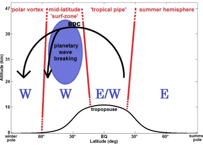
Figure 2.3: Schematic representation of the four regions of the stratosphere. The vertical red lines indicate barriers to horizontal mixing. The large blue letters indicate the dominant zonal mean zonal wind direction. A maximum in westerly winds separates the winter polar vortex and mid-latitude ‘surf-zone’ near 60°, while weak easterlies persist in the summer hemisphere. Zonal winds in the tropical pipe alternate between easterly and westerly (QBO, see also Fig. 2.6). Planetary wave breaking in the winter surf-zone (blue oval) results in poleward ‘pumping’ in the middle and upper stratosphere, which drives the Brewer-Dobson Circulation (BDC, black arrows). The diagram is based on Fig. 2 in Plumb (2002).

illustrated in Fig. 2.3. The tropical pipe is the only permanent feature, though its edges can shift considerably throughout the year (usually toward the summer hemisphere), while the other three regions depend on the season in their respective hemisphere.

[image:23.595.108.520.62.356.2]

(24)

from warmer, lower latitude air and allowing it to radiatively cool even further.2 _{The region}

between the polar vortex and the tropics is often referred to as the “surf-zone” (McIntyre and Palmer, 1984) since planetary wave breaking occurs regularly during winter and spring, causing considerable horizontal mixing in this region.

Planetary waves are planetary-scale disturbances that are created at the Earth’s surface by large-scale topography and the contrast in temperature due to differences in radiative heating over land and water. Under the right conditions, they can propagate upwards and transfer their momentum to the mean flow when they break in the stratosphere, making them an important source of momentum for the stratospheric circulation. Given the exponential decrease of density with altitude (Eq. 2.2), wave amplitudes increase as the waves propagate upward (due to energy conservation) and they eventually break, similar to water waves when they reach shallow water.

Rossby waves are a particular type of planetary wave that carry easterly momentum and for which the conservation of angular momentum acts as the restoring force. Charney and Drazin (1961) showed that Rossby waves with a zonal phase velocity c can only propagate vertically if the zonal wind, u, adheres to the inequality:

0< u−c < Uc (2.6)

whereUcis the Rossby critical velocity, which depends on latitude and the horizontal

dimen-sions of the wave. For typical Rossby wavelengths (≈10,000−35,000km) at mid-latitudes,

Ucis positive (westerly) with values of several tens of metres per second (Plumb, 2010). Since

the sources of these waves (large-scale topography and land-water contrasts) are permanent features of the Earth’s surface, atmospheric Rossby waves are often stationary with respect to the surface, i.e. their zonal phase velocity is zero. This simplifies Eq. 2.6 to:

0< u < Uc (2.7)

which is often referred to as the Charney-Drazin criterion (Holton, 2004). While Rossby waves are created throughout the year, Eq. 2.7 implies that they can only propagate into the stratosphere when the zonal winds are westerly (> 0) and not too strong (< Uc), e.g.

at mid-latitudes during winter and spring (Fig. 2.3). Similarly, the vertical structure of the zonal wind affects the altitude at which wave breaking occurs. As the zonal wind velocities tend to increase with height in the surf-zone, upward propagating waves eventually reach a critical level for which u = Uc. As the waves approach this level they begin to break,

depositing their momentum at or just below the critical level (Holton, 2004). The vertical range where the wavebreaking occurs is referred to as the critical layer.

Rossby wave breaking causes considerable horizontal mixing in the winter stratosphere. In summer, the persistent easterlies do not allow planetary wave propagation and horizontal mixing is relatively weak. The blue shaded region in Fig. 2.3 indicates the area in which most planetary wave breaking takes place. In addition to causing horizontal mixing, the easterly momentum deposited by breaking Rossby waves drives a poleward circulation known as the Brewer-Dobson Circulation (BDC;Shepherd, 2003). This circulation effectively sucks up

2_{The cold temperatures are also one of the main prerequisites for the formation of the ozone hole in the}

(25)

2.1. Atmospheric Structure and Stratospheric Dynamics

air from the tropical regions and pumps it toward the pole where it cools off and sinks. The continuous breaking of planetary waves, and the accompanying deposition of easterly momentum, also affects the springtime deceleration and eventual break-up of the polar night westerly jet. Due to the larger topographical contrasts, planetary wave activity is generally higher in the northern hemisphere, which is the main reason for the earlier break-up of the northern hemisphere polar vortex compared to the Antarctic one.

2.1.1 Stratospheric Tracers

More than 99.9% of the Earth’s atmosphere is made up of only three gases: nitrogen (N2,

78%), oxygen (O2, 21%), and argon (Ar, 0.93%). All other gaseous components of air

oc-cur in much smaller (trace) amounts. Gases that are also relatively chemically inert with respect to a particular timescale will be transported along with the atmospheric flow wi-thin that timescale and are therefore often referred to as chemical tracers. Their relative amounts are often given in volume mixing ratio with units of parts-per-million-by-volume (ppmv), parts-per-billion-by-volume (ppbv), or parts-per-trillion-by-volume (pptv), though other measures such as partial pressure or mole fraction are also common. The turbulent dynamics in the troposphere, and particularly in the boundary layer3_{, result in the air}

under-going thorough vertical and horizontal mixing on relatively short timescales (several weeks for intra-hemispheric mixing). Additionally, many trace species have tropospheric sources all over the globe, limiting the potential for latitudinal gradients. Accordingly, long-lived trace species are almost evenly distributed throughout the troposphere. The average time they spend in the atmosphere before they undergo a chemical reaction is much longer than the mixing timescale.

The considerably slower mixing processes in the stratosphere and the existence of distinct regions separated by mixing barriers, imply that large-scale circulation patterns, such as the BDC, have a significant effect on the distribution of the chemical constituents. Due to the slow large-scale dynamics, most chemical tracers are gradually removed with time. This means that the chemical composition of stratospheric air is dependent on the time the air has spent in the stratosphere.4 _{Depending on the lifetime of a particular chemical}

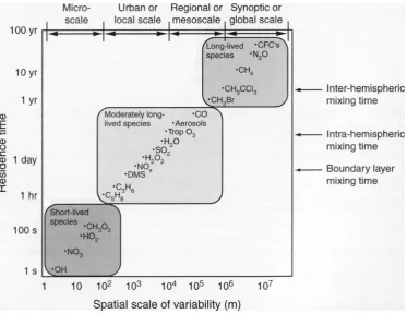
and the location of its stratospheric sources and sinks, different scales of mixing can be important in the spatial distribution of these tracers. Figure 2.4 shows the average lifetime of a number of atmospheric tracers on the vertical axis and the spatial scale on which their distribution varies on the horizontal axis. The stratospheric distribution of long-lived tracers with an average chemical lifetime of several months or even years, e.g. nitrous oxide (N2O)

or methane (CH4), are strongly influenced by large-scale, long-term circulation tendencies

such as the BDC (which has an overturning time of about three years; Rosenlof, 1995). In reverse, this implies that the large-scale distribution of a long-lived tracer can be used to infer details about the underlying dynamics occurring in the stratosphere. This is illustrated by the zonal mean distribution ofN2O for October shown in Fig. 2.5. Figure 2.5 is derived from

observational data from the Earth Observing System Microwave Limb Sounder (EOS-MLS) which is discussed in more detail in Sect. 2.3.3. Among other chemicals, the EOS-MLS

(26)

Figure 2.4: Atmospheric trace gas residence times and associated mixing scales (fromWallace and Hobbs, 2006).

observes three stratospheric tracers: nitrous oxide (N2O), methyl chloride (CH3Cl), and

carbon monoxide (CO), which are used in the present work. The main chemical processes that affect the stratospheric abundances of these tracers are detailed in the following.

Nitrous oxide is created at the Earth’s surface by biological processes as well as human activities. It is relatively evenly distributed throughout the troposphere with an average mixing ratio of approximately 320 ppbv (Lambert et al., 2007). The main source of stra-tospheric air in general and strastra-tospheric N2O in particular is in the tropics. The intense

surface heating in this region causes deep convection whereby the air rises rapidly and can penetrate through the tropopause. At higher latitudes, mixing from the troposphere into the stratosphere is generally reduced and occurs intermittently (Stohl et al., 2003). Once it has reached the tropical lower stratosphere, the up-welling arm of the BDC causes the air with its (high) tropospheric amounts of N2O to move upward and eventually poleward, which is

why the peak of each contour in Fig. 2.5 is found in the tropics. When the air reaches higher altitudes, the increase in short-wave solar radiation enhances the photodissociation of N2O

according to Eq. 2.8:

N2O+hν −→N2 +O (2.8)

where hν represents a photon of ultra-violet (UV) light (λ < 337 nm; Bates and Hays, 1967). The amount of UV light is much higher in the upper regions of the stratosphere than at lower levels, as it gets absorbed by the ozone layer between 20 and 30 km altitude. Hence, the chemical lifetime of N2O is only a few months at 40 km (≈ 1400 K) compared to 100

[image:26.595.90.464.61.349.2]

(27)

2.1. Atmospheric Structure and Stratospheric Dynamics

5 5 10 10 10 30 30 50 50 70 70 90 110 130 150 170 190 210 230 250 270 290 300 Latitude (deg)

Potential temperature (K)

80S 60S 40S 20S EQ 20N 40N 60N 80N 400 600 800 1000 1200 1400 1600 1800

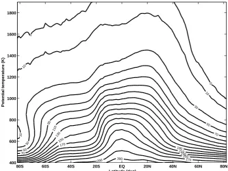
Figure 2.5: Meridional cross-section of zonal mean nitrous oxide (N2O) mixing ratio (contours

in ppbv) for October from combined satellite measurements from 2004 to 2011. The strong horizontal gradients near 20°S and 60°S are associated with the transition regions between the tropics, surf-zone, and the polar vortex. The potential temperatures from 400 to 1900K

approximately correspond to a vertical range between 16 and 47 km altitude (compare Fig. 2.2).

(Eq. 2.8) is its main stratospheric sink (Lambert et al., 2007), though the chemical reaction with excited oxygen radicals (O):

N2O+O −→2N O (2.9)

also occurs frequently at high altitudes and further reduces the N2O abundance.

Conse-quently, the mixing ratio of N2O gradually reduces with time while the air is pumped

po-leward by the BDC. In the winter mid-latitudes (between approximately 20°S and 60°S in Fig. 2.5), the strong horizontal stirring caused by planetary wave breaking results in a flat-tening of theN2O contours. This creates a meridional gradient between the tropics and the

surf-zone that can be seen as a step in the zonal meanN2O distribution (Fig. 2.5). Another

meridional gradient is observed between the winter mid-latitudes and the inside of the polar vortex (at approximately 60°S). Air from the surf-zone cannot easily penetrate through the strong winds of the polar night jet. Therefore, a large part of the air within the polar vortex is air that has been moved poleward at high altitudes by the BDC and has subsequently undergone cooling and descent. Accordingly, vortex air contains relatively low amounts of

N2O as most of it has been removed at high altitudes by the processes described in Eqs. 2.8

and 2.9.

Methyl chloride (CH3Cl) is a tracer similar to N2O in that it is created at the Earth’s

[image:27.595.150.484.63.313.2]

(28)

2.4) – which is shorter than that ofN2O but still sufficiently long to be useful as a tracer of

the dynamics in the lower stratosphere. Its typical volume mixing ratio in the troposphere is 600 pptv, almost three orders of magnitude smaller than that ofN2O.

In the stratosphere, Carbon monoxide has an even shorter average residence time than

CH3Cl. However, its chemical lifetime and abundance is highly altitude dependent. In the

mesosphere, CO is created through photolysis of carbon dioxide (CO2):

CO2+hν −→CO+O (2.10)

by high-energy UV radiation (hν) and CO’s lifetime increases from several months in the lower mesosphere to more than a year at higher levels (Jin et al., 2009). In the stratosphere,

CO is created during the photochemical oxidation of CH4 according to Eq. 2.11 (Randel

et al., 1998).

CH4+ 3O2+hν −→2H2O+CO+O3 (2.11)

The main sink of CO is oxidation by the hydroxyl radical (OH):

CO+OH −→CO2+H (2.12)

As the chain of reactions that lead to the creation of OH requires UV radiation (Eq. 2.13) and OH is very reactive, almost no OH is found in the polar middle atmosphere during winter due to the lack of sunlight.

O3+hν −→O2+O

O+H2O −→2OH

(2.13)

Therefore, there is little destruction ofCO during polar night andCO can accumulate inside the polar vortex during this time. In the presence of sunlight, however, the stratospheric lifetime of CO can be as short as three weeks in the upper stratosphere and as long as six months in the lower stratosphere (Jin et al., 2009). As a tracer, the unusual geometry of sources and sinks makes CO more dependent on local dynamics and seasonal effects than N2O and therefore can be a complimentary source of information on mixing dynamics,

particularly in the polar regions during winter.

2.1.2 Isentropic Potential Vorticity

Another quantity that is frequently used to analyse stratospheric dynamics is Ertel’s isen-tropic potential vorticity, often just referred to as potential vorticity (PV). It has properties very similar to chemical tracers in that it is conserved on potential temperature surfaces under the assumption of adiabatic motion. In isentropic coordinates the potential vorticity is defined as (Hoskins et al., 1985):

P V =−g(f_∂p+ζθ)

∂θ

(29)

2.1. Atmospheric Structure and Stratospheric Dynamics

where g is the acceleration due to gravity5_, _p _{is pressure,} _θ _{is the potential temperature,}

f is the Coriolis parameter, and ζθ is the isentropic vorticity. The Coriolis parameter is a

function of latitude, ϕ, and the Earth’s angular velocity, Ω = 7.2921·10−5 rad

s , according to

Eq. 2.15.

f = 2·Ω·sinϕ (2.15)

The isentropic vorticity, ζθ, depends on the horizontal wind field on isentropic levels:

ζθ =~k·

~

∇θ×~v

= ∂v ∂x ! θ − ∂u ∂y ! θ (2.16)

where~kis a vertical unit vector perpendicular to potential temperature levels, and~v = (u, v) is the horizontal wind vector, with uand v corresponding to the zonal and meridional wind component on isentropic levels, respectively. _∂x∂ and _∂y∂ are the derivatives with respect to longitude and latitude, respectively, where the index θ indicates that the derivatives are to be taken on potential temperature levels. The SI units of PV are m_{s kg}2K, but it is usually given in potential vorticity units or PVU, where 1 PVU = 1·10−6 m2_K

s kg .

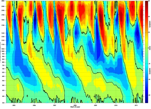
2.1.3 The Equatorial Quasi-Biennial Oscillation

Figure 2.6 shows a contour plot of the zonal mean zonal wind velocities at the equator from August 2004 through April 2011, derived from MERRA reanalysis data (see also Sect. 2.3.2) on potential temperature levels. Negative wind velocities (blue) correspond to easterly winds, positive velocities (red/yellow) are westerly. The thick black contour indicates the zero wind line. Figure 2.6 illustrates that the zonal mean wind does not follow a strictly seasonal or annual variation, particularly between 400 and 1250K.In this region the zonal winds oscillate between downward propagating easterly and westerly winds with an approximately two year period. The long-term average period is 28 months, but the actual period can vary between 22 and 34 months (Baldwin and Dunkerton, 2001). Hence this zonal wind pattern is known as the (equatorial) quasi-biennial oscillation (QBO). Above 600K,the QBO’s easterly phase tends to last longer and the westerlies descend faster, while the opposite is the case between 600 K and the tropopause.

The QBO is the result of the interaction of different types of atmospheric waves with the zonal mean flow. The waves are similar to Rossby waves (see Sect. 2.1) but can carry either westerly or easterly momentum. Waves that carry westerly momentum can only propagate upwards when the zonal winds are easterly, while those that transport easterly momentum can only propagate upwards when the prevailing winds are westerly (Baldwin et al., 2001). When these waves break in the stratosphere they transfer their momentum to the background flow, thereby decelerating the zonal winds which allow them to propagate in the first place. This feedback effect causes the cyclic behaviour of the QBO. Figure 2.7 illustrates this mechanism. In Fig. 2.7a, the average zonal wind profile in the stratosphere, u(thick line), is

5_g_{= 9}_.₈ m

s2 is assumed, independent of altitude. Whileg can vary by up to 2% between the surface and

(30)

[image:30.595.44.533.202.553.2]

(31)

2.1. Atmospheric Structure and Stratospheric Dynamics

westerly at lower levels but changes rapidly to easterly with altitude,z. Waves with a westerly phase velocity (+c) cannot propagate far into the stratosphere as they can only propagate upwards when the background winds are easterly. Waves with easterly phase velocity (−c) on the other hand, can propagate through the lower part of the stratosphere until they reach a critical layer where the average zonal wind velocity is easterly and similar in magnitude to the phase velocity of the wave (i.e. when |u−c| is small), where they break and deposit their easterly momentum (double arrow in the left half of Fig. 2.7a). The critical layer tends to lie below the altitude where cmatches ¯u, which means that the maximum descends with time.6_{Above the maximum there are no further driving forces and viscous diffusion gradually}

reduces the mean zonal winds (thin horizontal arrows in Fig. 2.7). Similarly, the thinning layer of westerly winds at the lowest levels is eventually destroyed by viscous forces when it becomes too thin (Gray, 2010). The resulting purely easterly mean wind profile (Fig. 2.7b) now allows waves with westerly phase velocity to propagate upwards. When these break at higher levels, they speed up the deceleration of the prevailing easterlies. Eventually, this results in increasingly westerly winds at higher levels impeding the vertical propagation of the westerly momentum carrying waves while at the same time the peak in easterly winds moves further down (Fig. 2.7c). Now the westerly wind regime gradually descends, due to the breaking of the westerly momentum carrying waves, resulting in the reverse of the initial situation – thinning, low-level easterlies and westerly winds at higher levels (Fig. 2.7d). From here the cycle continues in reverse.

Figure 2.7: Illustration of the mechanism driving the QBO. Zonal wind velocities are shown on the horizontal axis. The thick lines indicate the background zonal wind profiles, the wavy arrows show how high waves with easterly (-) and westerly (+) phase velocity c can propagate. Double arrows correspond to acceleration driven by breaking waves, single arrows indicate the natural diffusive tendency of the atmosphere to slow down strong winds through viscous forces. After Baldwin et al. (2001) and Plumb (1984).

6_{This also explains how the downward propagation of the phase of the QBO can be driven by upwardly}

(32)

Figure 2.8: “Schematic diagram showing the zonal wind structure in the winter hemisphere in the westerly phase of the QBO in the lower stratosphere (top) and in the easterly phase (bottom). The dashed line in the bottom panel shows the location of the zero wind line. The thick arrows denote the dominant paths of wave activity propagation for quasi-stationary planetary waves forced near the surface in the extratropics” (from Hamilton, 1998).

Holton and Lindzen (1972) established that the waves in Fig. 2.7 carrying westerly mo-mentum correspond to planetary Kelvin waves, while mixed Rossby-gravity waves provide the easterly momentum. However, the QBO mechanism described here is only a simplified model. For example, the momentum provided by Kelvin and mixed Rossby-gravity waves has to be complemented by a “broad spectrum of gravity waves that account for the remaining accelerations” (Yang et al., 2011), the exact details of which are not yet fully understood. A more complete description of the QBO theory is given inBaldwin et al.(2001) and references therein, and a detailed explanation of the properties of the different wave types involved can be found in Holton (2004).

(33)

2.2. Tracer Data Processing with Rényi Entropy (

RE

)

the QBO is associated with more vigorous horizontal mixing in the surf-zone and a weaker polar vortex due to an increase in wave activity. This effect was discovered by Holton and Tan (1980) and is therefore also known as the Holton-Tan effect.

2.2 Tracer Data Processing with Rényi Entropy (

RE

)

The Rényi entropy (RE), as used here for atmospheric analysis, is a measure of the chemical information content of the area under consideration. It is similar to the idea suggested by

Sparling (2000) of characterising hemispheric probability density functions (PDFs) by using the Shannon entropy to define an “effective number of states” (Sparling, 2000) analogous to thermodynamics. A highly variable region, with a large number of air parcels containing different concentrations of a particular tracer, has a high entropy, since the tracer distribution has a detailed chemical structure. On the other hand, low entropy is associated with (almost) equal tracer concentrations everywhere, representing a field without any chemical structure (Sparling, 2000).

The RE statistical measure was introduced by Alfréd Rényi as a generalised form of the Shannon entropy information metric (Rényi, 1961). It can be written as:

RE(α, b, N) = 1 1−α ·ln

b

X

i=1

pα_i(b, N)

!

(2.17)

where pi(b, N) represents a discrete probability density function (PDF) derived from a

his-togram withN data points andb bins, andα is the exponent of theRE. Forα= 1, Eq. 2.17 converges to the Shannon entropy (Beck and Schlögl, 1993).7 _In _{Krützmann et al.} ₍₂₀₀₈₎

and Krützmann (2008) it was shown that the RE can be applied to PDFs derived from chemical tracer fields of a chemistry-climate model, in order to identify tracer gradients that are associated with barriers to horizontal mixing. Specifically, the standardised8 _RE _with

α= 2 was used to identify the mixing barrier at the Antarctic polar vortex edge in ten years of SOCOL model simulations of stratospheric methane (CH4).9 This standardised form of

the RE is given in Eq. 2.18:

RE(2, b, N) = − 1

ln(b) ·ln

b

X

i=1

p2_i(b, N)

!

(2.18)

This form of the RE will also be used in the following, unless explicitly mentioned other-wise. It can be considered as a measure of the homogeneity of a PDF, i.e. how evenly the probabilities are distributed among all possible values. The maximum RE = 1 corresponds to a perfectly flat PDF – all values are equally likely.

7_For_α_→_{1 the}_RE _{converges to the Shannon entropy. This can be seen by applying l’Hôpital’s rule to}

Eq. 2.17.

8_The_RE _{given in Eq. 2.17 can be standardised by dividing it by the maximum possible value, which is}

the logarithm of the number of bins used, ln(b).

9_The_RE _{is a monotonically decreasing function of}_α _{and other values of} _α_{could be used as well, but}

(34)

The probabilities that make up the PDFs,pi(b, N), are calculated by binning the chemical

tracer mixing ratios within a particular region into a histogram withb equal-width bins and dividing the population of each bin by the total number of points N in the histogram.10 _In

order to create a reliable representation of the local tracer distribution, zonal concatenation of data points is often performed, i.e. all data points at a particular latitude are used to create the histogram for that latitude. When considering large-scale dynamics in the stratosphere, daily variations in tracer concentrations at a given altitude can usually be neglected since vertical transport is relatively slow. Therefore, several days of data can be combined to further increase the number of points for creating the PDFs. In the following, the method of creating the PDFs is indicated by a subscript where appropriate. For example, when using ’zonal ten-day PDFs’, i.e. including all data points at a particular vertical level and latitude from ten consecutive days, this is abbreviated as REz10. Other data windows used

for creating atmospheric tracer PDFs include combining zonal data from ten days and three latitude bins (REz10la3), or combining the data from five latitude and nine longitude bins

(REla5lo9).

The basic idea behind using the RE is as follows: a stratospheric barrier that prevents horizontal mixing (or slows it down considerably) will lead to a meridional gradient in the distribution of long-lived (relative to the mixing timescale) chemical trace gases to build up across the barrier (Miyazaki and Iwasaki, 2008). On either side of such a barrier, mixing can occur relatively unhindered, and randomly selected parcels of air are likely to contain very similar amounts of the chemical tracers present. Accordingly, a histogram (or PDF) of the concentrations of a particular tracer created from a sample of air parcels in such a well-mixed region can be expected to have a single strong peak close to the average mixing ratio of the tracer in this region, which drops off rapidly. If a histogram is created from data near the mixing barrier, however, air parcels with a range of tracer mixing ratios between the maximum on one side and the minimum on the other side of the barrier are likely to be present. Therefore, such a histogram is likely to be generally flatter and contain a much weaker peak with long tails or have multiple small peaks. As PDFs with strong peaks tend to have relatively low values of RE and flat distributions have high11_RE_{, tracer PDFs created}

from well-mixed air masses have low values of REwhile air close to a mixing barrier is likely to result in higher values of RE. This is illustrated in Fig. 2.9 which shows a meridional profile of the REz10 between 550 and 1450 K for 18.10.2008 (i.e. using data from 9th to 18th

October) calculated from satellite observations of N2O volume mixing ratios gridded to a

1.5° latitude grid and interpolated to potential temperature levels (for more details on this data set see Sect. 2.3.3), together with the histograms for six locations marked A through F. The ten-day zonal data window results in most histograms having between 280 and 290 data points, which should be a sufficiently large number to obtain a reliable representation of the local tracer distributions. The blue dotted lines are zonal mean N2O contours (in ppbv)

averaged over the same time period.

A broad comparison between the RE pattern and the zonal meanN2O contours shows

10_{As any histogram can be transformed into a PDF in this manner, the two terms are considered}

synony-mous in the following.

11_{The maximum} _RE _{value of one corresponds to a perfectly flat distribution, i.e. a PDF where all values}

(35)

2.2. Tracer Data Processing with Rényi Entropy (

RE

)

Figure 2.9: Meridional profile of the REz10 for 18.10.2008 (using data from 9th October to

18th) calculated from global satellite observations of N2O volume mixing ratios gridded to

a 1.5° latitude grid and interpolated to potential temperature levels. The blue dotted lines are zonal mean N2O contours (in ppbv) averaged over the same ten days. The histograms A

to F show the data used for calculating the RE value at the corresponding locations. The numbers in the top right corner of the histograms are (from top to bottom) the calculated

REz10 value, the corresponding latitude, the potential temperature level (in K), and the

Analysis of Internal Boundaries and Transition Regions in Geophysical Systems with Advanced Processing Techniques

Department of Physics and Astronomy, University of Canterbury,

Private Bag 4800, Christchurch 8140, New Zealand