Exploring the demand for bus transport : An exploration of the factors that determine the demand for bus transport and the development of a bus demand model

Exploring the demand for bus transport

An exploration of the factors that determine the demand for bus transport and the

development of a bus demand model

Master thesis

[Final report]

Marijn Smit

Exploring the demand for bus transport

An exploration of the factors that determine the demand for bus transport and the

development of a bus demand model

M.W. Smit BSc

Civil Engineering and Management University of Twente

marijnsmit@gmail.com

Supervisors:

Prof. Dr. Ing. K.T. Geurs University of Twente

Ing. K.M. van Zuilekom University of Twente

Dr. Ir. M.E. Kraan Grontmij

Ing. C. Doeser Grontmij

i

Abstract

Introduction

The challenge for bus operators is to optimize the supply of bus transport to demand as cost effective as possible. This demand is however not static; it depends on the supply of bus transport, population characteristics, urban developments, etc. In order to optimize the supply of bus transport, detailed information is needed about the impact of bus transport, population and spatial characteristics on demand. This thesis explores the factors that determine the demand for bus transport and uses those factors to develop a model which is able to predict the number of boarders and alighters at a bus stop and assigns them to the bus network.

Methodology

A four step model approach is followed to create bus demand models, including the stages trip generation, distribution and assignment. A literature study is performed to identify the factors that determine the demand for bus transport. Data from different sources are used to represent those factors. The data of these variables are collected for the catchment area of each bus stop in Breda. Veolia Transport supplied chipcard data of Breda and Tilburg which are used to create the trip generation models via regression analyses. Also the variation of the number of passengers over time is analyzed. For the distribution step, distribution functions are calibrated for weekdays (Monday to Friday), Saturdays and Sundays.

Results

The factors that determine the demand for bus transport can be categorized in the categories population characteristics, spatial characteristics, bus service characteristics and trip specific characteristics, although many factors are related to multiple categories. The research showed that the demand for bus transport is mainly explained by the presence of the central station, the number of stops that can be reached from a stop without transfer, the floor area of offices and shops and the number of students at higher educational institutes.

Six trip generation models are developed for Breda: boarders and alighters weekday (Monday to Friday), boarders and alighters Saturday and boarders and alighters Sunday. The models perform quite well for Breda, but worse for Tilburg. The calibrated top log-normal distribution function is well able to reproduce the observed trip length distribution of both Breda and Tilburg. The combination of the trip generation and distribution models result in an average difference of 16% with the observed number of passengers at the busiest line segments in Breda, while this is 34% in Tilburg.

Conclusion

ii

Summary

Introduction

The challenge for bus operators is to optimize the supply of bus transport to demand as cost effective as possible. This demand is however not static; it depends on the supply of bus transport, population characteristics, urban developments, etc. In order to optimize the supply of bus transport, detailed information is needed about the impact of bus transport, population and spatial characteristics on demand. The recent introduction of the public transport chipcard and the availability of more detailed socio-economic and spatial data offer opportunities to gain more insight in the factors that determine the demand for bus transport. This thesis explores the factors that determine the demand for bus transport and uses those factors to develop a model which is able to predict the number of boarders and alighters at a bus stop and assigns them to the bus network.

Research design

The objective of this research is to explore the factors that determine the demand for bus transport and implement these characteristics in a model that is able to predict the number of boarders and alighters at a bus stop and use those to predict the number of bus passengers in the bus network.

The developed model is a four step model with the stages trip generation, trip distribution, modal split and assignment. The third stage -the modal split- is not considered, since it is a unimodal demand model. Figure 1 shows the procedure of the development of the four step model.

iii

Literature

The factors that influence the demand for bus transport which were found in literature can be categorized in the categories spatial characteristics, population characteristics trip specific characteristics and bus service characteristics. Examples of factors are age, population (size), ethnicity (population characteristics), college enrolments, number of jobs, density (spatial characteristics), trip purpose (trip specific characteristics), accessibility, fare and quality of service (bus service characteristics).

Data assessment

Data from several sources are used to represent the factors that were found in literature. The main sources are the Centraal Bureau voor de Statistiek (CBS) for population characteristics, Dienst Uitvoering Onderwijs (DUO) for education related indicators, OpenStreetMap for the roads, buildings and bus stop locations, Kadaster for the data about addresses (Basisregistratie Adressen en Gebouwen) and Veolia Transport for the chipcard data.

Most of the data is available at the spatial levels 4-position postcode, neighbourhood, squares of 500m and squares of 100m. All spatial data which is used is converted to the squares of 100m, since this is the spatially most detailed level. The last stage of data processing is the collection of the data within the catchment area of 200 meters of each bus stop.

Veolia Transport provided the chipcard data of Breda and Tilburg of 2012. This data contains the hourly number of boarders and alighters at each bus stop in Breda and Tilburg in 2012. These datasets were used to create the trip generation models. Veolia Transport also provided data about the yearly number of passengers between each bus stop pair in Breda and Tilburg in 2012, divided in yearly number of passengers on weekdays (Monday to Friday), yearly number of passengers on Saturdays and yearly number of passengers on Sundays. None of the available chipcard data contains information about transfers.

Variation over time

The percentage of boarders during each month is approximately 7.7-10.8% of the yearly number of boarders, except for July and August with only 3.9 and 5.3%. Of all bus passengers, 90% travel on weekdays with an equal distribution over the weekdays (Monday to Friday), 6.3% travel on Saturdays and the remaining 3.7% travels on Sundays. Holidays have a quite large impact on the number of bus passengers: during the holiday weeks in 2012 the weekly number of boarders is about half of the average number of boarders. Although there is a morning peak on weekdays between 8:00 and 9:00h, during a period of four hours in the afternoon the hourly number of passengers is equal to or higher than during the morning peak.

iv Generation models

Six trip generation models are developed: boarders and alighters weekday (Monday to Friday), boarders and alighters Saturday and boarders and alighters Sunday. First, from all 67 explanatory variables the variables are selected which have a significant correlation with the dependent variable (e.g. boarders on weekdays) at both Breda and Tilburg. Via an iterative process the variables are selected which are included in the final generation models. Table 1 shows the variables which are included in the six trip generation models.

Table 1: Variables of the six trip generation models

Variable Boarders Alighters

weekday Saturday Sunday Weekday Saturday Sunday Number of stops without

transfer      

Dummy for Central station      

Percentage low income

households      

Floor area of offices      

Floor area retail, social gathering and

accommodation

     

Address density      

Total number of cars      

% of floor area with

residential function  

Number of students at higher

education institutes  

Dummy for University (of

Applied Science)  

Dummy for shopping centre (>5000 m2 floor area retail, social gathering and accommodation)

   

Distribution models

While the trip generation models determine the number of boarders and alighters at each bus stop, distribution models are used to determine how many passengers there are at each bus stop pair with a direct connection. Three distribution models have been created: one for weekdays, one for Saturdays and one for Saturdays. For each time period three distribution functions are calibrated from which the best one is selected. The top log-normal function is selected, since it is almost perfectly able to reproduce the observed trip length distribution. Validation

Nine models have been developed for Breda: six trip generation models and three distribution models. The generation models are validated for Breda and Tilburg, the distribution models are validated for Tilburg and the combination of the generation and distribution models are validated for both Breda and Tilburg.

v

performance of the models. At Saturdays and Sundays, the differences between the observed and modelled numbers are much larger. The distribution models perform slightly worse when applied to Tilburg, but they also match the observed trip length distributions very well.

The combination of the trip generation and trip distribution models perform very well for Breda. The cumulative average difference between the observed and modelled number of passengers is only 16% at the line segments with at least 1,000 passengers and increase to 40% at the busiest half of the linesegments. For Tilburg the differences are 34% at the line segments with at least 1,000 observed passengers and 66% at the busiest half of the line segments.

Conclusion

The demand for bus transport can mainly be explained by spatial factors, like the presence of the central train station, offices, shops and higher education institutes. These spatial factors represent facilities that attract a relatively large number of passengers. Other factors that are important are the accessibility indicator (number of stops that can be reached without transfer), the address density, percentage of low income households and the total number of cars.

The trip generation and distribution models are developed for Breda and perform quite well for Breda, but worse when applied to Tilburg. The worse result in Tilburg is mainly caused by the generation models. Since the models perform worse for Tilburg than for Breda, it can be concluded that bus demand models developed for one area cannot simply be applied to another area. Very specific combinations of circumstances have a large influence on the developed models, which is emphasized by the high sensitivity of the models for the sample of bus stops.

Recommendations

Larger study area

Very specific combinations of circumstances appeared to have a large influence on the trip generation models. Therefore more research is necessary to identify the variables that determine the demand for bus transport in general. An analysis with more municipalities might show why a variable is correlated with the number of passengers in one municipality and not in the other.

Use more detailed chipcard data

The chipcard data contains more detailed data than used in this study, like the number of passengers per bus line, the travel product people use to pay for their bus trip and the daily number of passengers between each bus stop pair. Using this more detailed data could provide more insight in improve the developed models.

Add explanatory variables

vi

Preface

This Master’s thesis concludes my study Civil Engineering and Management at the University of Twente in Enschede. It is the result of eight months of internship at the mobility department of Grontmij in De Bilt.

The start of the graduation process was quite a challenge. Finding subjects was not really an issue: there were plenty of interesting topics. After a selection process, a few topics related to bus transport remained. These topics raised an issue: finding data of public transport in general is difficult, but for bus transport this is even harder. Attempts of myself to gain access to chipcard data came to nothing, but luckily Cees Doeser found Veolia Transport willing to supply chipcard data. None of my supervisors had experience with the possibilities and limitations of this relatively new data source however, so also the design of the research was a challenge.

Finally, the research could begin. At some point, the research went so smooth, that Kasper van Zuilekom challenged me to extend the scope of the thesis. Until that moment I only considered the number of boarders at each bus stop, but now I also considered the distribution of the bus passengers over the bus stops and the number of passengers at the bus lines. Although some extra months were necessary because of the extended scope, I am happy with the added value it has to the thesis.

There are some people who I would like to thank. First I would like to thank Rob Kooloos and Piet van den Bosch of Veolia Transport for the supply of the chipcard data. I would also like to thank them for sharing their knowledge of the chipcard data and the bus system in general. I would like to thank my supervisors at Grontmij Mariëtte Kraan and Cees Doeser for their feedback and assistance. I also would like to thank Kasper van Zuilekom, my daily supervisor, for the joined-up thinking about the research and the discussions about the reports and Karst Geurs for the feedback on the reports. Finally, I would like to thank my family for supporting me.

vii

Table of contents

1 Introduction ... 1 1.1 Public transport in The Netherlands

1.2 Study area

2 Research design ... 6 2.1 Research objective

2.2 Research questions 2.3 Operationalisation

3 Model development ... 8 3.1 Four step model

3.2 Direct demand model 3.3 Model choice

3.4 Conclusion

4 Literature review ... 14 4.1 Spatial characteristics

4.2 Population characteristics 4.3 Bus service characteristics 4.4 Conclusion

5 Data assessment ... 21 5.1 Population characteristics

5.2 Bus service characteristics 5.3 Spatial data

5.4 Chipcard data 5.5 Conclusion

6 Processing of data ... 28 6.1 Checking consistency data

6.2 Creating additional variables 6.3 Conclusion

7 Comparison of Breda and Tilburg ... 33 7.1 Spatial characteristics

7.2 Population characteristics 7.3 Bus service characteristics 7.4 Conclusion

8 Data analysis: variation over time ... 37 8.1 All bus stops together

8.2 Bus stops separately 8.3 Effect holidays and events 8.4 Effect weather

8.5 Conclusion

9 Development generation models ... 46 9.1 Preparation regression analysis

9.2 Creating trip generation model boarders weekday

9.3 Compare included variables with literature and other models 9.4 Conclusion

10 Distribution analysis ... 57 10.1 Analysis of distribution in Breda

10.2 Calibration procedure 10.3 Results

10.4 Sensitivity of models 10.5 Conclusion

viii 11.1 Procedure of assignment

12 Validation ... 66

12.1 Validation trip generation models 12.2 Validation distribution models 12.3 Conclusion 13 Sensitivity analysis ... 76

13.1 Sensitivity significant correlations 13.2 Sensitivity regression coefficients 13.3 Conclusion 14 Conclusion ... 80

14.1 Answering sub research questions 14.2 Main conclusion 14.3 Recommendations for further research 15 Literature ... 87

16 List of appendices ... 91

Appendix I Detailed data description ... 92

Appendix II Effect of events on the number of bus passengers ... 94

Appendix III Weather characteristics ... 96

Appendix IV Input variables regression analysis ... 97

Appendix V Insignificant variables correlation analysis ... 99

Appendix VI Creating regression models ... 101

Appendix VII Comparing model variables with other models ... 102

Appendix VIII Calibration procedure distribution functions ... 104

Appendix IX Create distribution models for weekend ... 106

Appendix X Validation regression models ... 109

Appendix XI Validation distribution models ... 110

1

1

Introduction

People that want or need to travel have several transport modes to choose from. People living in large urban areas can choose for the bicycle, car and several types of public transport like train, metro, tram or bus. People living in rural areas are usually restricted to bicycle, car and sometimes bus. Travelling is quite easy for people that choose for the bicycle or the car: the road network is always available and offers only limited restrictions. For people that choose for public transport the story becomes more complicated, since the supply of public transport is both time and space restricted. If the supply of public transport is not properly aligned with the transport demand, it will be more attractive for people to use the bicycle or car.

Train, tram and metro operators only have limited tools to align supply with demand, since they are bounded to fixed infrastructure. The bus system however is more flexible, because it is only to a limited extent bounded to fixed infrastructure. The challenge for bus operators, municipalities and concession holders is to optimize the supply of bus transport to meet the demand as cost-efficient as possible. This demand is however not static, it depends, among others, on the supply of public transport, population specific characteristics and urban developments. Because of changing population characteristics in neighbourhoods it might be that other bus routes are more effective.

Before the national introduction of the public transport chipcard (finished in 2012), the NVS counts were the main source of information about the number of passengers in the buses. These counts were only spot checks performed during two weeks in March or November, which resulted in very rough estimations. The estimations were rough because of potential counting (or estimation) errors and because of the limited number of counting days. These counts are therefore not suitable to optimize the supply of bus transport. Because of the lack of detailed data, it was not known which effect urban and demographic developments have on the number of bus passengers. The chipcard data however offers detailed information about the number of boarders and alighters per hour at each bus stop and the origin and destination stops.

2

1.1

Public transport in The Netherlands

1.1.1

Concession areas

Since 2001 the 19 regional public transport authorities are obliged to tender the public transport in their areas. In that year the new law that manages public transport in the Netherlands came into force: the “Wet Personenvervoer 2000”. The transport company that wins the tender is granted the exclusive right to provide the regional public transport in the concession area for a certain period of time. Figure 2 shows the 45 concession regions, which are granted to 13 transport companies (Kennisplatform Verkeer en Vervoer, 2013).

Figure 2: Concession areas in the Netherlands at January 1st, 2014. Adapted from Kennisplatform Verkeer en Vervoer, 2013.

1.1.2

Chipcard system

Since 1980 passengers could pay for their journey with public transport with the

3

number of passengers nor about their travel behaviour (e.g. board and alight stops). To gain some insight in the number of passengers each year during a few weeks the NVS counts (Normeringssysteem Voorzieningenniveau Streekvervoer) were conducted in March and/or November. At each bus line some counting stops were appointed. At those bus stops the bus driver counted the number of bus passengers in the bus (Directoraat Generaal van het Verkeer, 1981). This system gave some insight in the number of passengers at that moment, yet only a rough indication. It gave however no information about the origins and destinations of those passengers nor about the number of passengers in other periods. The central organisation of the sales of the strippenkaart also resulted in difficulties with the distribution of the turnover over the operators. A complex system, the WROOV system (Werkgroep Reizigers Omvang en Omvang Verkopen), was needed to determine which fraction of the sales belonged to each operator (Centrum Vernieuwing Openbaar Vervoer, 2004).

Another disadvantage of the strippenkaart was the tariff structure, namely through zones. Since the tariff depended on the number of zones a passenger passed, the size and location of zone borders had much influence on the costs of travelling with public transport. This way a short trip could be more expensive than a long trip, just because of the zone layout.

From 2007 the new chipcard system was introduced gradually. In this new system the

strippenkaart was replaced by a system with chipcards, requiring passengers to check in and check out (Van der Zwan, 2011). This provides detailed information about the boarding and alighting stops, travelled distance and allows spatial and temporal tariff differentiation. The chipcard system is maintained by Trans Link Systems (TLS), a joint venture of public transport operators. All transactions between passengers and the transport operators go through TLS. Since the chipcard system enables detailed information collection, there is a strict privacy policy. Because of this policy, not all information that is collected by the chipcard system can be accessed by the transport operators. Because of this, TLS does not provide information about the transfers of public transport passengers to the operators, creating an empty space in their data.

Data which is available are the number of boarders and alighters per bus line per bus stop, aggregated per hour. It also shows information about the travel product that is used to pay (e.g. credit, student subscription, age discount, etc.) and the distances travelled. It is however not possible to identify individual passengers to see for example how their travel behaviour over multiple days is.

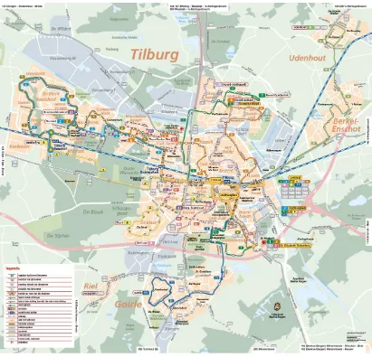
1.2

Study area

4 the stadium of Breda’s football club NAC. Breda has two train stations: Central station (intercity station) and Breda-Prinsenbeek (regional train station).

Figure 3: Bus lines in the municipality of Breda. Reprinted from Veolia Transport (2012).

5

6

2

Research design

This chapter elaborates on the design of the research. It first gives the research objective. The second section shows the research questions and the third section explains the methodology that is used to answer the research questions.

2.1

Research objective

With more insight in the factors that influence the demand for bus transport, transport planners are able to optimize the exploitation of their bus system and adapt the system on changes in urban development. Therefore the influences of the factors that determine the number of boarders and alighters and their impact on the number of boarders and alighters at a bus stop need to be explored. The aim of this study is therefore to explore the factors that determine the demand for bus transport and implement these characteristics in a model that is able to predict the number of boarders and alighters at a bus stop and use those to predict the number of passengers in the bus network.

2.2

Research questions

The main research question of this study is:

Which factors determine the demand for bus transport and how can these factors be implemented in an explanatory model that is able to predict the number of boarders and alighters at a bus stop and used to predict the spatial distribution of those passengers?

In order to answer the main research question and meet the research objective, the following sub questions are composed:

1. How can bus demand be modelled according to the theory and what are the requirements of the model for this study?

2. Which factors determine the demand for bus transport according to the literature?

3. Which indicators can represent the factors that were found in the second research question and which data is available about these indicators?

4. How does the number of bus passengers vary over time?

5. How can the number of boarders and alighters at bus stops be predicted using a model? 6. How can the distribution of bus passengers over the network be modelled?

7

2.3

Operationalisation

1. How can bus demand be modelled according to the theory and what are the requirements of the model for this study?

A literature review has been performed about some examples of different types of models that are used to model the demand for public transport. With these model types in mind, the setup of the models that are developed in this study is given.

2. Which factors determine the demand for bus transport according to the literature?

A literature study has been conducted in order to gain insight in the factors that determine the demand for transport, with a focus on bus transport. This has resulted in an overview with the most important factors that determine demand for bus transport.

3. Which indicators can represent the factors that were found in the first research question and which data is available about these indicators?

In order to include the factors that influence the demand for bus transport that were found in research question 2, indicators are needed that represent those factors. The availability of data about those indicators and suitability to consider in this study were checked.

4. How does the number of bus passengers vary over time?

The variation of the number of bus passengers over time are explored, as well as the influence of certain weather characteristics and the effect of large events in the study area.

5. How can the number of boarders and alighters at bus stops be predicted using a model?

The indicators that influence the demand for bus transport and the chipcard data are combined in a regression model which is able to predict the number of boarders and alighters at bus stops.

6. How can the distribution of bus passengers over the network be modelled?

For this research question a Gravity model is produced by calibrating distribution functions. The distribution functions should be able to produce an origin-destination matrix with a given number of boarders and alighters at bus stops.

7. How valid are the developed models?

8

3

Model development

In order to support decision making, a bus demand model is developed. This model should be able to forecast the number of boarders and alighters at the bus stops and determine the destinations of the bus passengers. Socio-economic data is used to explain the number of boarders and alighters which is retrieved from the chipcard data. There are two types of aggregated models that are potentially suitable for these purposes. The first is the classic four step model, which is actually a collection of four models: trip generation model, distribution model, modal split model and the assignment model. The second model type is the direct demand model. The direct demand model combines the trip generation and distribution and modal split models in one model: the demand of each origin-destination pair is determined per mode. The two types of models are discussed in the following three sections. In the final section a choice is made for the most suitable model type with more elaboration on the model development.

3.1

Four step model

The four step model is a general, often used approach to determine the amount of traffic on links in the transport network. Although it origins from the 1960’s, it is still a common approach. Figure 5 shows the four stages of the model. The first step, the generation stage, determines the number of trips that start and end in each zone. In this study it determines the number of boarders and alighters at each bus stop in a particular time period. The second stage determines how the boarders and alighters are distributed over the bus network, so how many people travel between each pair of bus stops. This results in an origin-destination matrix. (Ortúzar and Willumsen, 2001)

9

1. Generation

2. Distribution

3. Modal split

4. Assignment

Flows

Figure 5: The classic four step model

3.2

Direct demand model

The direct demand model is somewhat similar to the four step model, but it combines the trip generation, distribution and modal split stages in one model. Socio-economic characteristics of the catchment areas of both the boarding and alighting stop are combined in the model, as well as trip specific characteristics. The result is an origin-destination matrix with the number of passengers on the bus stop pairs with a direct bus connection. Once the origin-destination matrix is created, the passengers can be assigned to the bus network. (Ortúzar & Willumsen, 2001)

3.3

Model choice

From the four step model and the direct demand model the four step model is assumed to be most appropriate for this study. The separate models for the trip generation and distribution stage allow more insight in the functioning of the stages. At the start of the study it was not yet known how well the demand for bus transport could be estimated by demand models, so the separate models offers some flexibility. The four step model offers more manual control, e.g. if the trip generation model estimates a number of boarders at a bus stop that is obviously much too low, it is possible to manually change the number of boarders before proceeding to the distribution stage. This kind of flexibility is not offered in the direct demand model.

10 The aggregated basis of both models has some disadvantages. It is for example hard to implement trip specific characteristics, such as travel time and accessibility. Both models do not model behaviour and are therefore unable to model the effect of policy and changing travel behaviour (Domencich & McFadden, 1975).

Because of the advantages of the four step model over the direct demand models, a four step model is developed. The following subsections elaborate the development of the four step model.

3.3.1

Generation

The most common approach of determining the number of trips generated by and attracted to each zone is by using socio-economic data. The generation models can be produced with a regression analysis. Some aspects need to be addressed in order to produce the generation models: The factors that determine the demand for bus transport, the variation of the number of bus passengers over time, the number of boarders and alighters at the bus stops and the catchment area of bus stops.

1. The factors that determine the demand for bus transport

In order to identify the factors that determine the demand for bus transport a literature study is performed. The literature study provides a list of variables that are important for the demand for bus transport. The second step is to explore the availability of data about these factors and explore the availability of additional data that might be relevant. The final stage is to process and prepare the data for the trip generation models.

2. The variation of the number of boarders and alighters over time

The variation of the number of bus passengers over time is explored by creating figures of the number of boarders per time period. The time periods that are assessed are months of the year, weeks of the year, days of the week and hours of the day. Next to these time periods the influence of holidays and events are explored as well.

3. The number of boarders and alighters at the bus stops

The observed number of boarders and alighters at the bus stops per time period is necessary to create the trip generation models. This data is available through the chipcard data.

4. The catchment area of bus stops

The literature study also addresses the catchment area of bus stops that is found in other studies. Apart from this, stepwise regression models are created for several catchment areas to see which catchment area gives the best regression model. The catchment area with the best fitted regression model is assumed to be most suitable.

Once these four subjects are addressed, the generation models can be produced. The following methodology will be followed for each trip generation model:

11

2. Select the variables that are significant in both Breda and Tilburg and identify other variables that are either significant in Breda or Tilburg or variables that are considered to be important.

3. Create a correlation matrix with these selected variables for both Breda and Tilburg 4. Remove the variables that are strongly correlated (≥ 0,5) with multiple other

variables

5. Create regression models for both Breda and Tilburg, remove variables that are insignificant in both Breda and Tilburg

6. Once all models are created, try to uniformize the models by adding and/or removing variables resulting in models with similar combinations of variables. E.g. there are five models with a variable ‘floor area of offices’ and one with a variable ‘number of offices’. Both variables are strongly correlated, so if the influence on the model is limited, the variable ‘number of offices’ is replaced with ‘floor area of offices’.

7. The developed models for Breda are the final models.

3.3.2

Distribution

There are several methods to determine the distribution of the passengers between the bus stops. The focus is either on the trip itself, using generalized costs, or on the activity that is the reason to travel. In this study, the focus is on the trip itself, since no information is available about the activities that are performed by the bus passengers. The most used method for trip distribution is the Gravity model, which uses travel costs to determine the impedance to travel between each pair of bus stops. The model assumes the willingness to travel to a particular bus stop only depends on those travel costs. Examples of travel costs are generalized costs (a combination of several costs), distance and travel time. The gravity model uses a distribution function (also known as deterrence function) that needs to be calibrated. The result of the distribution model is an origin-destination matrix.

An alternative for the gravity model is distribution with an intervening-opportunity model. The basic assumption of intervening-opportunity models is that people will travel to the destination which satisfies the aim of the trip which is closest by or best accessible. It works with the probability a destination is able to satisfy the objective. If there is a bus line which serves bus stops A to E (in order of serving) and a passenger travels from A to E, then apparently stops B, C and D cannot fulfil the objective of the journey although they are closer by. Calibrating the model determines the likelihood of each bus stop to satisfy the trip. This model is however quite complicated to compute and more difficult to understand than the gravity model. (Ortúzar & Willumsen, 2001)

In literature various distribution functions can be found, but since it is not feasible to examine all those functions, a few different functions need to be assessed. The function that gives the best results of the distribution is selected. The functions that are assessed are:

12

 Tanner function:

 Top log-normal function:

3.3.3

Assignment

The final stage of the four step model is the assignment of the distribution matrix to the bus network. In situations where the assignment of the traffic to the network influences the distribution (e.g. because travel times increase making other routes more attractive) an iterative procedure is recommended. In this study however, it is assumed people will take the shortest route (measured by number of bus stops). In reality there are several factors that determine which bus line people take, like frequency and directness of the route, but these are ignored in this thesis.

3.4

Conclusion

13

14

4

Literature review

The studies that examine the demand for bus transport on aggregated level can be categorized in two categories: those that focus on factors that explain the number of bus passengers and those that focus on factors that cause a change in demand for bus transport. Although there is an overlap between the factors in those categories, this study focuses on the first category and therefore the focus will be on studies from the first category. Those factors can be classified in the categories population characteristics, spatial characteristics, bus service characteristics and trip specific characteristics.

4.1

Spatial characteristics

Spatial characteristics are important factors that determine travel time and travel distances. Because of suburbanisation in the Netherlands the distances between residential areas and commercial and industrial areas are relatively large, which has a negative effect on bus transport demand (Steg and Kalfs, 2000). The spatial characteristics that influence the demand for bus transport can be discussed using the five D’s of development:

1. Density 2. Diversity 3. Design

4. Destination accessibility 5. Distance to transit

Density

Density is usually the number of people or employees per square kilometre. In high density areas more people live within the catchment area of public transport stops or stations, which allows more efficient public transport. According to several studies more trips are undertaken by public transport in high density areas (Campoli and MacLean, 2002; Lee and Cervero, 2007; Limtanakool, Dijst and Schwanen, 2006).

Diversity

Diversity of land use, like mixed land use, especially influences demand for transport for non-work related trips (Lee and Cervero, 2007). Mixed land use allows people to walk or cycle towards their destination instead of having to travel a longer distance (Cervero and Kockelman, 1997), although this might have a negative effect on the demand for bus transport. Lee and Cervero (2007) found that a good mix of residents and jobs reduces vehicle trips.

Urban design

The urban design of the environment of a bus stop needs to facilitate the access routes for bus passengers. Most bus passengers travel to the bus stop by walking or cycling, which can be supported by offering direct and save routes between the origins and destinations of the passengers and the bus stops, in other words: offering a pedestrian and cyclist friendly environment (Lee and Cervero, 2007).

Destination accessibility

15

important factor. When the destination is well accessible from the bus stop (e.g. at a walkable distance), the bus will become more attractive to use. Destination accessibility can be described to be the number of activities like jobs, parks, shops that can be reached within some amount of time (Ewing, Meakins, Bjarnson and Hilton, 2011).

Distance to transit

The circle theory assumes there is a maximum distance people are willing to travel to access a transit stop or station. The theory is that people living closer to a bus stop are more likely to travel via that bus stop than people living further away. In the Netherlands, this radius is usually presumed to be about 500 meters, because this is found to be the maximum distance people are willing to walk to a stop (Van der Blij, Veger and Slebos, 2010). There is however not an unambiguous distance that can be used in this study, so this needs to be investigated.

4.2

Population characteristics

Ethnicity

Ethnic minorities make other choices in travelling than Dutch natives. The bicycle ownership among Moroccans, Surinamers, Antilleans and Turks is far lower than that of Dutch natives, namely a quarter of these minority households do not own a bicycle, while this is 3% for natives. The minorities travel less by bicycle and car and more with public transport. In similar situations, when natives choose to use the bicycle, minorities choose for public transport. Possible explanations are cultural differences (differences between men and women, low social status of bicycle) and a relatively large number of people who never learnt to cycle (Harms, 2006). It might also be influenced by the location where ethnic minorities live, e.g. in higher density neighbourhoods in the vicinity of well served bus stops. The number of ethnic minorities might therefore have a significant influence on the demand for bus transport. Also Taylor, Miller, Isekia and Fink (2008) showed the number of recent immigrants have a large influence on the demand for bus transport.

Age

For certain age categories age has a large influence on demand for bus transport. Other than one might expect, elderly (65+) do not use the bus more often than other people, yet the category 80+ make 3% of their trips with the bus compared to 2% for the whole population (Bakker, Zwaneveld, Berveling, Korteweg & Visser, 2009). Balcombe et al. (2004) however found that the bus accounts for 12% and 13% of the trips of respectively the age groups 70+ years and 17-20 years. Since the group of 70+ is small, the total influence of this group on the demand for bus transport is limited. Pupils and students in the Netherlands make about 29% of their trips with public transport and are therewith an important age group to consider.

Income & car ownership

Income mainly has an indirect effect on bus transport demand. Income has a very large impact on car ownership and availability, which is a major factor in bus transport demand (Balcombe et al., 2004). People that do not own or have access to a car depend on other ways of transport, like public transport, cycling or walking. Taylor et al. (2008) showed the number of households without a car influences the demand for bus transport.

16 people that do and do not have a car available. The figure shows that the group of people in the Netherlands that do not have a car available travel significantly more with public transport. For this group, public transport can be considered to be important, but their share in the total number of passenger kilometres is fairly limited (Bakker et al., 2009).

Figure 7: Modal distribution of the number of passenger kilometres for people that do and do not have a car available in the Netherlands. Adapted from Bakker et al., 2009.

Bicycle ownership

Approximately 84% of the Dutch people own at least one bicycle (Fietsersbond, 2011). Bicycles are however also an important competitor for bus transport, since both operate on relatively short distances. The average bus, tram and metro journey in the Netherlands is about nine kilometres from stop to stop, while figure 08 shows that the bus, tram and metro (BTM) have a very small share of trips shorter than 7.5 km.

Figure 8: Modal choice for trips shorter than 7.5km in the Netherlands. BTM = Bus, tram and metro. Adapted from Fietsersbond, 2011.

4.2.1

Trip specific characteristics

Trip purpose

17

transport is significantly lower for commuter trips, viz. 14%. Of the total number of vehicle kilometres of bus, tram and metro, 33% is made for educational purposes and 30% is commuter traffic. Other purposes are visiting people, shopping and other social activities (Bakker et al., 2009). Although the trip purpose is hard to operationalize for this study, there are some indicators that are related to those purposes, like population (home based trips), college enrolments (educational trips) and number of jobs (commuter trips). Taylor et al. (2008) found the latter two to have a significance influence on the demand for bus transport.

Travel time

The travel time is the time that is needed to travel from the origin to the destination. The travel time of public transport is often longer than that of private vehicles, since the public transport is usually not from door to door, other than for example cars or bicycles. The travel time of bus transport not only consists of the in-vehicle travel time, but also the access- and egress time and the waiting time. According to Balcombe et al. (2004), the amount of time that people spent travelling is more or less constant at a value of about one hour. This means that the longer the access- and egress time and waiting time are, the less time people are willing to spend in a vehicle. This means that the actual area that can be reached with the bus is smaller than with the car.

Factors that are important in travel time are the directness of the route, the necessity to interchange or not and the distance between the origin and the boarding stop and the destination and the alighting stop.

4.3

Bus service characteristics

Fare

Fare has to be paid to make usage of a bus service, with exception of cases where bus transport is free for particular groups. Taylor et al. (2008) found that the fare levels of bus services have a large influence in the number of passengers. The fare levels do however not differentiate within the study area and is therefore not included in this analysis.

Quality of service

The quality of service is used to measure the performance of a public transport service. A service with a good performance has a better quality of service than services with a low performance. The quality of service can be determined using different factors that all together determine the quality of service. It can be measured using objective and subjective indicators and some indicators have both an objective and a subjective value, for example the punctuality (Eboli and Mazzulla, 2011). The objective indicators are measurable and unambiguous (assuming objectivity exists), while the subjective indicators reflect the judgments of travellers about those indicators. If only subjective indicators are used, the indicators together result in a perceived quality of service.

18 minutes between two consecutive buses. A higher frequency results in a higher bus demand, since waiting time is reduced resulting in a lower total travel time.

Rojo, Gonzalo-Orden, dell’Olio and Ibeas (2012) found that bus characteristics (i.e. the quality of the bus) only influence demand for bus transport for long distances (> 15km), although it does influence user satisfactory for all trips. According to Paulley et al. (2006), the conversion of high-floor buses to low-floor buses results in a demand growth of about 5%. This increased demand would come from people in a wheelchair, people with small children and people with a lot of luggage. Another example of a bus characteristic that is important to some people is the presence of a functioning air-conditioning system (Eboli and Mazzulla, 2011). Another factor that impacts the quality of service is whether people have to interchange or not. People do not like to interchange on their journey, although the degree in which it influences the demand for bus transport depends on the waiting time during transfer (Balcombe et al., 2004). Another major factor is the total length of the journey; people are less dissatisfied about transferring at longer journeys than at short ones (Wardman, 2001). The value of the transfer is found to be between 4.5 and 30 in-vehicle-minutes (Guo, 2003). The value of a transfer in the Netherlands is approximately 11 minutes (Oostra, 2004 via Goudappel Coffeng, n.d.).

The reliability of a bus service is the ability to hold on to the schedule and to depart and arrive at the desired locations at the planned moments (Eboli and Mazzulla, 2011). An unreliable bus service results in longer waiting and travel times for passengers and hence will dissatisfy them and decrease demand for bus transport. Since busses usually don’t stop at stops where no passengers desire to leave or board the bus, this causes some unreliability in bus services.

The final factor related to the quality of service discussed here is the provision of information. Information can be provided online, at the bus stops and in the bus itself. Usually the information includes the timetable, but the availability of information about delays is increasing. According to Grotenhuis the most desired pre-trip information is the total travel time, interchanges and real time delay information. The most desired roadside information is real time delay information, trip advice and the departure platform (Grotenhuis as cited by Grotenhuis, Wiegmans and Rietveld, 2007). Nearly all bus stops in the Netherlands are fitted with a time table and the number of digital passenger information systems with current departure times is growing.

19

Reputation

Several studies have shown that the bus has a rather bad reputation among people (Pommer, Van Kempen and Eggink, 2008; Tertoolen and Van Uum, 2004). It is remarkably that frequent bus users rate the bus higher than not-users. The bus services in the Netherlands received ratings of 7.1 to 8.3, which show that bus users actually are quite satisfied with the bus services (Kennisplatform Verkeer en Vervoer, 2013). Because of a lack of appropriate data this factors is not considered in this study.

4.4

Conclusion

The literature study came up with several factors that influence the demand for bus transport. These factors can be divided in four categories: spatial characteristics, population characteristics, trip specific characteristics and bus service characteristics. Figure 9 shows the four categories in relation to the bus system. It shows the boarding and alighting stop, each with a catchment area. The catchment area of the boarding stop has spatial and population characteristics while the alighting stop only has spatial characteristics. The bus service and trip characteristics are related to the connection between the two stops.

Figure 9: The four categories of factors that influence the demand for bus transport in relation to the bus system.

Where

Hk,x,y = boarding stop k with coordinates x and y

r = radius of the catchment area of the bus stops Sk,spatial = spatial characteristics of bus stop k

Sk,population = population characteristics of boarding stop k

Sk,trip = Trip specific characteristics from boarding stop k

Sk,bus service = bus service characteristics from boarding stop k

Hl,x,y = alighting stop l with coordinates x and y

20 Table 2 shows the characteristics in the four categories spatial characteristics, population characteristics, trip characteristics and bus service characteristics. Some factors can be categorized in multiple categories, but are assigned to one category. There are two factors which are only applied to the alighting stop: college enrolments and number of jobs. These two factors are typical destination variables. People that board the bus at a specific bus stop, will usually return to that bus stop later in the day. Therefore no distinction is made between boarding and alighting stop.

Table 2: Factors that influence the demand for bus transport according to the literature. The boarding stop contains factors in four categories, while the alighting stop only has one category of factors.

Boarding stop Alighting stop

Spatial Population Trip Bus service Spatial

Density Age Trip purpose Quality of service

College enrolments

Distance to bus stops

Population Travel time Fare Number of jobs

Urban design Income/car ownership

Reputation Distance to bus stops

Diversity Bicycle ownership

Accessibility

21

5

Data assessment

The previous chapter concluded with an overview with factors that influence the demand for bus transport according to the literature. In order to include those alternatives in the regression analysis, indicators about those factors need to be available. This chapter examines several data sources and the available data that represent the factors from literature. The first section assesses the data which is available about the population characteristics. The second section describes the data which is available about bus service characteristics and the third section shows the available spatial data. The final section presents the chipcard data which is available for this study.

5.1

Population characteristics

5.1.1

Centraal Bureau voor de Statistiek

The Dutch Statistics Agency (Centraal Bureau voor de Statistiek, CBS) has data available about various socio-economic characteristics on different spatial levels. The three spatial levels which are relevant for this study are:

 Neighbourhood

 Squares of 500m

 Squares of 100m

Since the study focuses on 2012, data from 2012 should be used. Some useful or necessary data is however not (yet) available for 2012, so for those variables the data of 2011 is used. In case data about variables is available on different spatial levels, the spatially most detailed level is used. In those cases the consistency of the data is checked (see section 6.1).

22 Figure 10 shows some of the 56 neighbourhoods in the municipality of Breda. Since the study focuses on 2012, data of 2012 is used. The data for 2011 contains however more variables than the data of 2012, of whom a few are considered relevant for this study. The following data (2012) from CBS on neighbourhood level is considered to be relevant (CBS, 2013):

 Total number of cars

 Average number of cars per household

 Percentage of western foreigners

 Percentage of non-western foreigners

The variables in the data of 2011 that is not available yet for 2012 but is considered to be relevant are the following (CBS, 2012):

 Number of social security eligibilities (bijstandsuitkeringen)

 Average distance to school with VMBO (following the road)

 Average distance to school with havo or vwo (following the road)

 Average distance to a train station (following the road)

Figure 11 shows the municipality of Breda with squares of 500m, containing data from CBS. The data at this spatial level from the CBS that is considered to be relevant for this study are (CBS, 2013):

 OAD (omgevingsadressendichtheid, average address density)

 Percentage of low income households

 Percentage of high income households

23

Figure 12 shows the municipality of Breda with squares of 100m containing data about several socio-economic characteristics. The following characteristics are selected (CBS, 2013):

 Number of people

 Number of people 0-14 years

 Number of people 15-24 years

 Number of people 25-44 years

 Number of people 45-64 years

 Number of people 65 years and older

 Percentage of western foreigners

 Percentage of non-western foreigners

5.1.2

Municipality of Breda

The municipality of Breda has information available about the number of jobs in every neighbourhood in Breda (breda.buurtmonitor.nl). The data is available for the years 2003 to 2012. Other data that is available from the municipality that might be relevant and complements the data from CBS is the average income per household on neighbourhood level. The most recent data that is available is from 2009, but according to CBS the average disposable income in Noord-Brabant in 2012 was more or less equal to 2009, namely 0.3% lower (statline.cbs.nl). It is assumed this difference is similar in Breda. The variables from the municipality of Breda that will be used are:

 Number of jobs

 Average disposable income (2009)

24

5.1.3

Dienst Uitvoering Onderwijs

Dienst Uitvoering Onderwijs (DUO), the Education Executive Agency of the Ministry of Education, Culture and Science publishes education related data on their website (DUO, n.d.). Data from DUO that has been selected for this study are the following:

 Number of pupils per 4-position postcode

 Number of pupils per school (secondary education)

 Number of pupils per intermediate vocational educational institute (MBO)

 Number of students per university of applied science (HBO)

 Number of students per university (WO)

5.2

Bus service characteristics

The bus service characteristics are obtained from two primary sources: Veolia Transport and OpenStreetMap. Information about the routes of the bus lines and the travel times are obtained from the busboekjes with the timetables and the bus stops per bus line, from the website of Veolia Transport and from the line maps. The locations of the bus stops are obtained from OpenStreetMap, which is an open source mapping project.

5.3

Spatial data

25

Figure 13: Map of Breda city centre and Breda West including the addresses and their function. The white circles represent addresses with the function 'woon' (residential), purple the function 'winkel' (retail) and red the function 'bijeenkomst' (social gathering). © Kadaster

5.4

Chipcard data

For this study chipcard data of 2012 is used, which is supplied by Veolia Transport. Four chipcard data sets are used. The first dataset contains the number of boarders and alighters per hour per bus stop per bus line in Breda in 2012. Both urban and regional bus lines are included. The set contains 331 excel files: 28 bus lines with a separate file for each month (some lines do not operate during July). The second dataset contains the number of passengers between each pair of bus stops per bus line in Breda that have a direct bus connection, summed over the year. This set contains 70 excel files: 28 bus lines with a separate file for the weekdays (summed), Saturdays and the Sundays. Not each bus line operates during the weekend, so not each bus line has three excel files.

26

Figure 14: Screenshot of one of the chipcard datasets. It shows the number of boarders and alighters per hour per bus stop at bus line 1. Each bus stop has two columns, the left column contains the number of boarders during the hour and the second column contains the number of alighters. © Veolia Transport

The third data set contains the number of boarders and alighters per hour per bus stop per bus line. The set contains 240 excel files: 20 bus lines with a separate file for each month. The fourth file contains the number of passengers between each pair of bus stops per bus line in Tilburg that have a direct bus connection, summed over the year. This set contains 57 excel files: three excel files per bus lines (one for the weekdays, one for Saturdays and one for Sundays).

Figure 15 shows a screenshot of one of the excel files in the third dataset. It contains the number of passengers at some bus stop pairs of line 1 in Breda on all weekdays in 2012.

27

Although, or because, the datasets contain large amounts of data, some data is missing or wrong. The datasets do not contain information about transfers, so a journey from A to C with a transfer at B is registered as a trip from A to B and a trip from B to C. From the data it can not be deduced that the trips are connected with each other. Data at some bus stops during some time periods is missing and some bus stops are included twice, but with another unique number. The datasets with the boarding and alighting stops (like in figure 15) contain stops that are not served by that bus line, which need to be filtered out of the data.

5.5

Conclusion

This chapter assessed the data which is available about the factors that determine the demand for bus transport according to the literature study. For the population characteristics most data is obtained from the CBS, which has data available about for example the number of people per age category, ethnic groups and number of cars. The data is available at the spatial scales neighbourhood, squares of 500m and squares of 100m. Other population characteristics are obtained from DUO about education related factors and the municipality of Breda about income and the number of jobs.

28

6

Processing of data

The previous chapter presented the data that is used in this research. It showed that the data comes from different sources and at different spatial levels. The data needs to be fused to one layer with data. The data is processed using Quantum GIS, which is open source Geographic Information System software. Since a more detailed spatial level gives more detailed spatial information, which is beneficial for this study, the data is merged to the squares of 100m. In order to enable the data fusion, one major assumption needs to be made: it needs to be assumed that the characteristics are uniformly spread over the data object, e.g. a uniformly spread of the population within a neighbourhood. This assumption allows data fusion based on area. Figure 16 shows an example of how data about the population in a neighbourhood is converted to squares of 500m.

Figure 16: The distribution of a population of 1000 people over squares of 500 meter. The first figure gives the neighbourhood and the squares; the second figure gives the areas of the squares and neighbourhood; the third figure gives the proportion of the area which sums up to 1. The last figure gives the population per (part of the) square. The sum of these populations is equal to the population of the neighbourhood.

The first section checks the consistency of some variables which are available at multiple spatial levels. The second section elaborates on the creation of variables which need to be created from the available data or need additional processing.

6.1

Checking consistency data

Since some data is available on multiple spatial levels, the consistency of the data needs to be checked. The consistencies of the population and of the number or percentages of foreigners are checked in the following subsections.

6.1.1

Population

29

Figure 17: The number of occurrences of the differences in population between the 500m squares and the summed 100m squares. I.e. there are 136 squares of 500m with 5 more people than the summed population in the corresponding 100m squares and 27 squares of 500m with 10 people more than in the corresponding 100m squares.

6.1.2

Foreigners

The CBS data in the layers of 500m and 100m squares only offer percentages of foreigners in different categories (e.g. category 1: >67% western foreigners, category 2: 45-67% non-western foreigners, etc.). Only the data on neighbourhood level provides absolute numbers. Since the number of foreigners might be an important factor in the number of bus passengers, it is investigated if it is possible to use the data from 100m level. Table 3 gives an overview of the number of foreigners according to several sources. Since the data at the 500m and 100m squares are only in categories, the average of the categories are used to calculate the absolute number of foreigners (e.g. for a category of 10-20% foreigners 15% is used). For the last row the population of the 100m squares are used and the percentages of foreigners come from the neighbourhood level. It appears the combination of 100m squares and neighbourhood give a very good result, while it is spatially much more detailed than the data on neighbourhood level.

Table 3: Number of foreigners according to different sources

Source population

Source percentages

Western foreigners

Non-western

foreigners Dutch Total

CBS Statline - - 18.993 19.275 138.133 176.401

Municipality of

Breda - - 19.080 19.315 138.158 176.553

GIS (CBS)

Neighbourhood Neighbourhood 19.094 19.317 137.880 176.291

500m squares 500m squares 19.048 14.022 139.548 172.618

100m squares 100m squares 18.943 20.541 133.125 172.609

30

6.2

Creating additional variables

Although most of the data is ready to use, some relevant variables need to be created, either manually or using collected data. The following variables are created:

 Dummy variable for Central Station

 Dummy variable for higher education

 Floor area per function within catchment area

 Percentage of floor area per function (all floor area is 100%)

 Number of addresses per function within catchment area

 Floor area with shopping centre functions ‘winkel’, ‘bijeenkomst’ and ‘logies’

 Percentage of area per function

 Dummy variable for shopping centres

The creation of the dummy variables for Central Station and higher education is pretty straightforward: the dummy for Central Station has a value of 1 for the central bus station and value 0 for all other bus stops. The bus stops next to Universities and Universities of Applied Science have a value of 1 for the dummy variable for higher education, while the other stops receive a value of 0 for this variable. The BAG data is used to calculate the floor area and number of addresses per function within each catchment area. Figure 18 shows a part of Breda with the addresses and the total floor area per function per catchment area. The floor area per function within each catchment area is used to determine the percentage of floor area per function.

Figure 18: Map of Breda city centre and west of the city centre with the addresses in this area. The size of each pie diagram depends on the total floor area within the catchment area. © Kadaster