On the effect of a Gaussian firing rate function on the dynamics of a network of Wilson Cowan populations

Master Thesis

Faculty of Electrical Engineering, Mathematics and Computer Science (EEMCS)

On the effect of a Gaussian firing rate

function and propagation delays on

the dynamics of a network of

Wilson-Cowan populations

B. Kiewiet

Commitee:

Prof. Dr. S.A. van Gils

Dr. H.G.E. Meijer

Dr. J. le Feber

Abstract

C

ONTENTS

1 Introduction 5

2 Model Description 7

3 Dynamics with a Gaussian Firing Rate Function 9

3.1 A single E-I population . . . 10 3.2 Two coupled populations. . . 16 3.3 Multiple populations . . . 20

4 Dynamics with a Propagation Delay 23

4.1 Two coupled populations. . . 23 4.2 Multiple populations . . . 26

5 Discussion 29

C

HAPTER

1

I

NTRODUCTION

Worldwide almost 65 million people suffer from epilepsy, a neurological disease with charac-teristics that are currently difficult to understand. Epilepsy is a disorder characterized predom-inantly by recurrent and unpredictable interruptions of normal brain function called seizures, with a seizure a transient occurrence of signs and/or symptoms due to abnormal excessive

or synchronous neuronal activity in the brain [1]. The disease can roughly be divided into

two groups based on the type of seizures [2]: Generalized and focal epilepsy. Research into

the disease is carried out eitherin vitro(human or animal tissue) orin vivo(animal or clinical

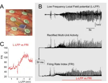
studies). Computational models can be of additional help in understanding the disease. A recent experiment that recorded local field potentials in the core of an epileptic focus using an array of micro-electrodes, showed a Gaussian relationship between the inverted low

frequency component of the potentials (L-LFP) and a multi-unit firing rate metric (Figure1.1).

Figure 1.1: Experimental recordings Based on these experimental results we want to

create a model that incorporates the Gaussian rela-tionship and analyze the fundamental changes in the dynamics as a result of this different relationship.

The brain consists of a large number of widely con-nected neurons, with short- and long-range connec-tions. Many models for individual neurons have existed

for some time (e.g. [3; 4; 5; 6]) and have been

ana-lyzed extensively (e.g. [7;8]). Since micro-electrodes

measures the activity of thousands of neurons the de-tails about individual neurons are omitted. Looking at a macroscopic level neurons form neuronal networks and epilepsy can be seen as the result of ”odd” activity

of an interconnected neural network [2]. Modeling this

experiment as a large number of neuron models is thus not required. Instead, Mean-field or neural mass models can be used to represent a large number of neurons. In this case results are more easily computed and interpreted than networks of a large number of single neuron models. With these type of models we look at the average behavior of populations of neurons.

Many different neural mass models have been created (e.g. [9; 10;11;12;13;14]) and are

most often described as nonlinear integral-differential equations. In this study we use the so called Wilson-Cowan equations as a basis to model our neural network.

Much mathematical analysis has been done on the equations since the model was first

published in 1972 [15]. A bifurcation analysis shows the different types of behavior and

bifur-cations this simple model has [16]. The Gaussian relationship between the L-LFP and firing

rate metric is modeled by switching the sigmoid for the Gaussian firing rate function in the equations. The firing rate function maps input current into a firing rate. Most neural mass mod-els assume that single neurons begin firing, based on a mean threshold and some variance

[17], and use a corresponding sigmoid or threshold firing rate function (e.g. [9;12;13]).

Mod-els for single neurons, however, show that with high input current, an individual neuron has a

depolarization block at which the neuron stops firing [7;18]. A Gaussian shaped firing function

effect of the shape of the firing rate function has been studied [19], but a Gaussian shaped function has not been used in this context.

Focal-onset start from a small region and spreads subsequently to other regions [1].

Addi-tionally, recent micro-electrode array recordings showed that propagation of neural activity

oc-curs at a spatial scale below the size of a conventional electroencephalogram (EEG) [20].This

justifies the use of a spatially extended network of multiple Wilson-Cowan populations to model the seizure in addition to a temporal evolution. Networks of populations have been studied (e.g

[21;22;23]) and showed spike-wave discharges and activity waves when networks were

spa-tially coupled.

A modification of neural networks is the incorporation of delays [24; 25; 26]. The finite

traveling speed of action potentials, transformations from electrical to bio-chemical signals and the spread of post-synaptic potentials in a neuron give reason to model spatially extended

systems with time delays [27]. It has been shown that a delay can generate new dynamics not

present without a delay. The micro-electrodes on the array are placed in a grid. We choose to incorporate a time delay in the model to represent the finite time an action potential needs to travel from one electrode on the grid to another.

In this study we look at a network of coupled Wilson-Cowan equations that uses a Gaussian firing rate function. The network has a propagation delay between populations and EEG output is modeled as the average current into three populations.

In chapter 2we give the mathematical model. In chapter 3we analyze the effect of using

a Gaussian firing rate function in a network without propagation delays. The effect of

incorpo-rating a propagation delay between populations is studied in chapter4. Finally, we discuss the

results in chapter5.

Research questions

In this study we try to answer the following questions:

• What is the effect of using a Gaussian firing rate function on the dynamics of the

Wilson-Cowan model?

• What is the effect propagation delays between excitatory populations on the stability of

periodic solutions in a network of Wilson-Cowan populations?

C

HAPTER

2

M

ODEL

D

ESCRIPTION

This study models a neuronal network as a set of coupled neural mass populations including spatial nearest neighbour interactions. Each local population is governed by the Wilson-Cowan equations, consisting of an excitatory and inhibitory subpopulation. The inhibitory tion receives self-inhibition in addition to an excitatory current from the excitatory subpopula-tion. The excitatory subpopulation receives self-excitation, an excitatory current from its neigh-bors and an inhibitory current from the inhibitory subpopulation. Each current has a strength

wX→Y that translates activity into current. Propagation delays between the excitatory

subpop-ulations is also incorporated. The Wilson-Cowan equations are given by:

E_k0 =−Ek+ (1−Ek)FE(JEk),

I_k0 =−Ik+ (1−Ik)FI(JIk),

wherek= 1...N and the Gaussian firing rate functions (FRF) are given by:

      

FE(JEk) = exp

−JEk−Eθ

Esd

2

−exp

−0−Eθ

Esd

2

,

FI(JIk) = exp

−JIk−Iθ

Isd

2

−exp

−0−Iθ

Isd

2

,

or in the sigmoid case:

FE(JEk) = (1 + exp (−EsSlope(JEk−Esθ)))

−1₋

(1 + exp (EsSlopeEsθ))−1,

FI(JIk) = (1 + exp (−IsSlope(JIk −Isθ)))

−1_{−(1 + exp (Is}

SlopeIsθ))−1,

with input currents,

JEk =wEEEk(t)−wIEIk(t) +αwEE(Ek−1(t−τ) +Ek+1(t−τ)) +B,

JIk =wEIEk(t)−wIIIk(t),

whereEkandIkare the activity of thekth excitatory and inhibitory subpopulations respectively.

The functionsFE(JEk)andFI(JIk)are the firing rate functions, which can be Gaussian shaped

or sigmoid, with as argumentJ the input current for the specific subpopulation. The constants

wEE, wEI, wII, wIE weigh the activity from the different sources. All excitatory subpopulations

receive the constant background currentB. An additional coupling strength between excitatory

subpopulations is given byα. The propagation delayτ between the excitatory subpopulations

is the time that it takes for a signal to reach it neighbors. In the first part of this study this delay

is zero. We model the EEG output as the average current. Figure 2.1 shows an schematic

E

I

E

I

E

I E

I

wEI wIE

wII

wEE

awEE

awEE

E

I

EEG

Figure 2.1: A schematic overview of the model. Each E-I pair is coupled, with or without

propagation delay τ, to its neighbors through its excitatory subpopulation. We model EEG

output as the average current over three populations. Solid: Excitatory connections; Dashed: Inhibitory connections.

Parameter Description Standard value Varies

wEE Weight of current between excitatory populations 16

wII Weight of feedback current of the inhibitory populations 3

wIE Weight of current from inhibitory to excitatory populations 12

wEI Weight of current from excitatory to inhibitory populations 18 x

Eθ Mean of Gaussian FRF of excitatory populations 7

Iθ Mean of Gaussian FRF of inhibitory populations 5

ESD Standard deviation of Gaussian FRF of excitatory populations 2.1

ISD Standard deviation of Gaussian FRF of inhibitory populations 1.5

Esθ Mean of sigmoid FRF of excitatory populations 5.2516

Isθ Mean of sigmoid FRF of inhibitory populations 3.7512

EsSlope Slope of sigmoid FRF of excitatory populations 1.5858

IsSlope Slope of sigmoid FRF of inhibitory populations 2.2201

B Background current of excitatory populations 2.45or3 x

α Connection strength between excitatory populations 0.1 x

τ Propagation delay between excitatory populations 0 x

Table 2.1: The parameter values are based on earlier modeling studies [9;10; 16;21]. The

C

HAPTER

3

D

YNAMICS WITH A

G

AUSSIAN

F

IRING

R

ATE

F

UNCTION

In this chapter we discuss the effect of a Gaussian firing rate function (FRF) on the dynamics of the Wilson-Cowan (WC) populations. In the original WC equations it was assumed that each individual neuron had a threshold after which a neuron would respond to excitation and start firing. Integrating the firing rate of individual neurons over the relevant domain yields a sigmoid population FRF. If we incorporate the effect of an upper threshold for depolarization block the corresponding population FRF is Gaussian shaped. Here we assumed that after the

upper threshold the individual neuron immediately stops firing. Figure3.1 shows this result.

Inhibitory cells are more easily activated than excitatory cells and thus the resulting firing rate functions are shifted to the left compared to the excitatory functions. The right figure shows the Gaussian and sigmoid functions used in our model. The parameters for the sigmoid are chosen such that the slope at the half activation point is identical to the Gaussian.

The WC equations are nonlinear and thus their dynamics can not be studied in the same way as with linear differential equations. In this report we use bifurcation theory to study the nonlinear Wilson-Cowan equations with a Gaussian FRF (WCG). Bifurcation theory in differen-tial equations looks at the qualitative structure of the dynamics. By using bifurcation theory on dynamical systems we try to find the parameter values at which behavior changes qualitatively.

For terminology and definitions of bifurcations we refer to [28]. A previous study computed a

bifurcation diagram, using a sigmoid FRF, with the background current and the coupling from the excitatory to inhibitory population as free parameters. Using these two free parameters is

adequate to describe the dynamics of a singleE −I pair. Indeed, with the background

cur-rent as a free parameter we can directly influence the excitatory subpopulation, while with the excitatory to inhibitory coupling we can influence the inhibitory subpopulation, independently from the background input. In line with this study we make a bifurcation diagram, using the

Matlab package Matcont [29], varying the same parameters and compare it to the bifurcation

diagram with the fitted sigmoid curve. Phase plane portraits are made, using Pplane8 [30], for

all regions with qualitative different behavior for the WCG equations. We use the bifurcation diagram and phase portraits to choose parameter values such that the effect of the Gaussian FRF is clear and oscillatory behavior is possible.

If two WCG populations are coupled, the interaction between them can generate new dy-namics. The coupling strength between two WCG populations determines the amount of activ-ity that is sent between the neighboring excitatory subpopulations. Bifurcation diagrams with the coupling strength as the active parameter are made for two cases with different background current. These diagrams will show the symmetry, stability and existence of equilibria and ex-trema of the periodic and quasi-periodic solutions. We study the effect of the Gaussian FRF on the dynamics of the coupled populations using time series and the bifurcation diagrams.

0 5 10 0

1

Input Current

Population FRF

0 1

Cell FRF

0 5 10

0 1

Input Current

Population FRF

0 1

Cell FRF

0 5 10

0 0.2 0.4 0.6 0.8 1

J

F(J)

Figure 3.1: Left: Heterogeneity in firing onset for individual cells leads to a sigmoidal population FRF. Middle: Including the effect of heterogeneous thresholds for depolarization block leads to a population FRF with a maximum. Right: The FRFs used in this paper. Solid: Gaussian; Dashed: Sigmoid; Blue: Excitatory; Black: Inhibitory

3.1

A single E-I population

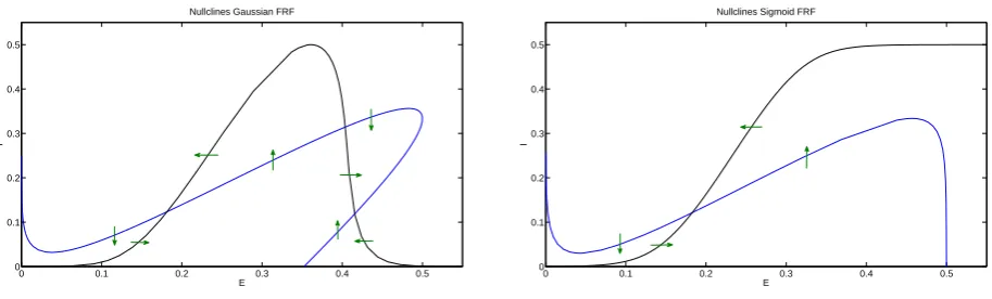
Here we look at a single E-I population. We first draw a comparison in the phase-planes of

the WCG and the WC equations with the parameter values from table 2.1. Figure3.2shows

the phase plane and their nullclines. The excitatory nullclines look similar in this region for the

chosen parameter values except that for high values ofEthe nullcline turns more sharply. The

inhibitory nullcline shows that with a Gaussian FRF the curve turns downward for high values

ofE. Due to this turn the inhibitory nullcline crosses the excitatory nullcline two more times

compared to the sigmoid nullclines. The two resulting equilibria do not exist in the sigmoid case. Of the two extra equilibria one is a saddle and the other a stable node. The stable node has high excitatory and low inhibitory activity. The saddle has both high excitatory and high inhibitory activity.

The additional steady state is a robust feature coexisting with the normal dynamic

reper-toire of the WC model with a sigmoid FRF. Figure3.3shows for three different values of wEI

bifurcation diagrams for varyingB with the excitatory activity on the vertical axis. The values

of wEI are chosen such that we cross several bifurcations in case B and C. In case A the

dynamics are similar to the dynamics with a sigmoid FRF, because the high activity equilibrium

does not exist for any value ofB in addition to the normal dynamic repetoire.

Case A

ForB <1.93the low activity equilibrium is the only equilibrium. AtLP1 two unstable equilibria

appear via a fold bifurcation. At SN IC another fold bifurcation removes the lower equilibria

and all orbits converge to a stable limit cycle. At H we have a supercritical Hopf bifurcation

and the limit cycle shrinks. AtLP3andLP2we have two fold bifurcations and afterward only a

0 0.1 0.2 0.3 0.4 0.5 0

0.1 0.2 0.3 0.4 0.5

Nullclines Gaussian FRF

E

I

0 0.1 0.2 0.3 0.4 0.5

0 0.1 0.2 0.3 0.4 0.5

Nullclines Sigmoid FRF

E

I

Figure 3.2: Nullclines and direction field for a Gaussian (left) and sigmoid (right) firing rate

function. Parameters as in table2.1withB = 3 andwEI = 18. Two additional high excitatory

activity states exist in the Gaussian case

low activity equilibrium exists. IncreasingBfurther the equilibrium converges to(E, I) = (0,0).

The bifurcation diagram can be found in figure3.3a.

Case B

ForB <−1.25the low activity equilibrium is the only equilibrium. AtLP1 we have a fold

bifur-cation and two high activity equilibria appear, of which the highest one is stable. Two unstable

equilibria come into existence at LP2 and at SN IC the lower stable equilibrium disappears.

All orbits then converge to a stable limit cycle or the high excitatory activity equilibrium. At

B = 4.693we cross a homoclinic bifurcation curve. An unstable limit cycle appears around the

stable limit cycle and both limit cycles disappear when we cross a limit point of cycles curve

(not indicated). At the fold bifurcationLP4 two unstable equilibria disappear and all orbits

con-verge to a high activity equilibrium. AtLP4 and LP5 we have two more fold bifurcations that

remove the high equilibrium and produce a low activity equilibrium respectively. If we increase

B further the equilibrium converges to(E, I) = (0,0). The bifurcation diagram can be found in

figure3.3b.

Case C

For B < −1.27 the low activity equilibrium is the only equilibrium. At LP1 we have a fold

bifurcation and two high activity equilibria appear. At fold bifurcation LP2 we have two new

unstable equilibria of which one immediately has a supercritical Hopf bifurcation atH1. AtLP3

two equilibria collide and disappear. Now all orbits converge either to the stable limit cycle or

the high excitatory activity equilibrium. The limit cycle disappears at H2 due to supercritical

Hopf bifurcation. AtB = 5.197we cross a homoclinic bifurcation curve and an unstable limit

cycle appears. At H3 we have a subcritical Hopf bifurcation that removes the unstable limit

cycle. The fold bifurcation LP4 removes the unstable equilibria and all orbits converge to a

high activity equilibrium. We have a new stable equilibrium at the fold bifurcationLP5 and at

the fold bifurcationLP6 the high excitation equilibrium is removed. If we increaseB further the

−20 0 2 4 6 8 10 12 14 0.1 0.2 0.3 0.4 0.5 B Min/Max E LP 3 H LP 1 LP 2 SNIC (A)

−20 0 2 4 6 8 10 12 14

0.1 0.2 0.3 0.4 0.5 B Min/Max E LP 1 LP 3 LP 5 LP₄ LP₂ SNIC (B)

−20 0 2 4 6 8 10 12 14

0.1 0.2 0.3 0.4 0.5 B Min/Max E LP 4 LP1 H 3 H₂ H 1 LP 2 LP 3 LP 6 LP 5 (C)

Figure 3.3: Bifurcation diagrams forwEI = 13(top),wEI = 18(middle) andwEI = 20.5(bottom)

with a Gaussian FRF. Blue: Stable equilibrium; Red: Extrema of limit cycles; Solid: Stable;

Dashed: Unstable. The dashed black line indicates a homoclinic bifurcation. By IncreasingwEI

a fold bifurcation is crossed and two high activity equilibria appear. The dynamics ifwEI = 13

Full Bifurcation Diagrams

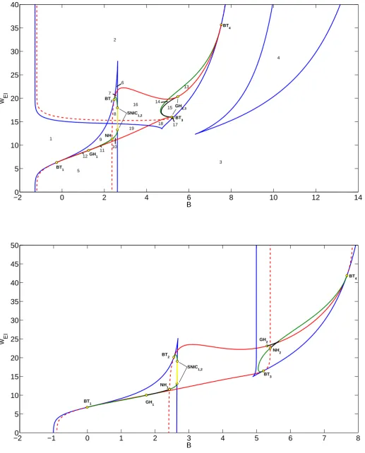
Figure3.4shows the bifurcation diagrams with background activityBand the coupling from the

excitatory to inhibitory populationwEI as free parameters. With these free parameters we are

able to show the main determinants of the dynamics, such as the existence of steady states and periodic oscillations.

For small values ofwEI the bifurcation diagrams of the WCG and WC equations look

sim-ilar. For large values ofwEI we find in the Gaussian case an extra fold (saddle-node) curve

that corresponds with the two extra high activity equilibria. At this fold curve we also find two Bogdanov-Takens points, which also exist in the sigmoid case but on a different fold curve

cor-responding to high values ofB. From the Bogdanov-Takens (BT) point a Hopf curve emerges

that ends at another BT point. On this Hopf curve there are degeneracies where the Hopf bifur-cation changes from super- to subcritical. Here limit point of cycle bifurbifur-cation curves emerges that end in points where the saddle along a homoclinic curve is a neutral saddle (NH). The homoclinic curves emerging from a BT point either end in saddle-node homoclinics (SNIC) or connect to another BT-point.

For the Gaussian case a characteristic phase portrait is created for all 19 areas, see figure

3.5. Starting from area 1, we find a single stable low activity equilibrium. Crossing the fold

bifurcation into areas 2 or 5 two equilibria appear. In area 2 they have high excitatory activity, while in area 5 the activity is low. Crossing another fold bifurcation into area 3 two equilibria collide and only a single stable equilibrium exists. In area 4 we have 3 equilibria with high excitatory and low inhibitory activity. In area 6 we find 5 equilibria of which 3 are stable. Going down into area 7 we cross a Hopf curve and a stable limit cycle appears with low activity. Into area 8 we go over a homoclinic curve and the limit cycle disappears. Down into area 9 we cross a fold curve and the two high excitatory activity equilibria collide and disappear. When we cross a homoclinic curve into area 10 a stable limit cycle appears. Crossing a homoclinic curve into area 11 gives rise to an unstable limit cycle around the stable limit cycle. Going from area 11 to 12 we cross a Hopf curve and the stable limit cycle disappears. In area 13 we find an unstable limit cycle and two high activity equilibria. Crossing the Hopf curve into area 14 a stable limit cycle appears inside the unstable cycle. Going into area 15 we cross a limit point of cycles curve and both limit cycles disappear. In area 16 we find a stable limit cycle and two high activity equilibria. Area 17 is equivalent to area 13 and crossing the homoclinic curve from area 17 into area 18 the unstable limit cycle disappears. In area 19 the only stable invariant

set is the limit cycle. The areas in one of the sets{1,3},{2,4,5,18},{9,15},{10,16},{11,14}

and{12,13,17}are all structurally equivalent. In total we have nine structurally different areas.

Effect of Gaussian FRF on a single population

The main effect of using a Gaussian FRF are the extra high activity equilibria in addition to the normal behavior we see in the original Wilson-Cowan equations. If the coupling strength

between the excitatory and inhibitory subpopulations (wEI) is large and the background input

B not too big, then the currentJI = wEIE −wIII is also large. The reverse is also true: If

wEI is small then the resulting current JI is also small. Due to the symmetric shape of the

Gaussian FRF and that wII is relatively small, the resulting firing rate will be similar for the

inhibitory subpopulation. This can be seen in the bifurcation diagram from the roughly similar shapes of the main curves and the large amount of structurally equivalent areas. Only areas 6,7 and 8 have low and high activity equilibria that coexist, because in those areas the main

bifurcation curves overlap. The effect of the Gaussian FRF is most clear forwEI = 18For this

−20 0 2 4 6 8 10 12 14 5 10 15 20 25 30 35 40 B w EI 10 1 2 6 7 5 3 4 14 18 12 11 13 8 17 BT₃ BT₄ GH₁ BT 1 BT 2 19 SNIC_1,2 NH 9 GH_2,3 15 16

−20 −1 0 1 2 3 4 5 6 7 8

5 10 15 20 25 30 35 40 45 50 B w EI

BT₁ GH

1 BT₂ BT₃ GH 2 BT₄ NH₁ NH₂ SNIC_1,2

Figure 3.4: Bifurcation diagrams for Gaussian (top) and sigmoid (bottom) firing rate function,

the active parameters are background inputB and coupling parameterwEI, other parameters

as in table2.1. Bifurcation curves are indicated with color: saddle-node (blue), Hopf (red), Limit

point of cycles (black), Homoclinic to saddle (green), Saddle node on invariant curve (yellow). The red dashed line indicates a neutral saddle curve, which is not a bifurcation curve. Note the

extra saddle-node curve for high values ofwEI and low values ofB and the different horizontal

3.2

Two coupled populations

Here we couple two populations by their excitatory subpopulations. We look at the impact of the coupling strength on the dynamics of the extended model. An extra parameter for the

coupling strength, denoted byα, is introduced. The input current into an excitatory population

then becomes: JEij = wEEEij −wIEIij +αwEEEji +B with i, j ∈ {1,2}, j 6= i. Based

on the analysis done for a single population we look at two cases: B = 2.45and B = 3, with

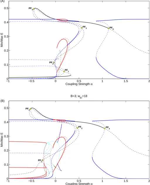
other parameter values as in table2.1. Figure3.6shows bifurcation diagrams with the coupling

strengthαas the free parameter and the activity of an excitatory population on the vertical axis.

Asymmetric branches forming from pitchfork bifurcations are linked, that is: If the upper branch

corresponds to the populationE1, then the lower branch corresponds to the other population

E2 and vice versa.

We distinguish between symmetric and asymmetric invariant sets, anti-phase and in-phase periodic solutions and quasi-periodic oscillations.

Case A

Here we useB = 2.45. In this case the parameter set for both single populations corresponds

to area 8 which has 5 equilibria of which two are stable. Activity from a neighboring population

can push a population into area 2 or 16 depending on the value ofα. Starting at the symmetric

low activity equilibrium (black line) for α <0we find atα = 0.332a fold bifurcation. Following

the branch we find atα = 0.181a pitchfork bifurcationP F1 which spawns two linked unstable

asymmetric equilibria. Continuing the symmetric branch we find at α = −0.038 a fold

bifur-cation. Shortly after we find P F2 at α = −0.035 which spawns another two linked unstable

equilibria. Atα = 0.115 we find a Hopf bifurcation (not indicated) which creates an unstable

symmetric limit cycle. We find atα = 0.607a fold bifurcation andP F3 atα = 0.555. The two

new linked branches have a Hopf bifurcation and create an unstable limit cycle at α = 0.292

before it disappears atα = 0.025due to a saddle-node homoclinic bifurcation. Continuing the

black symmetric branch we have at α = −0.484 a fold bifurcation and at P F4 the symmetric

equilibrium becomes stable again. Following the linked asymmetric equilibria we have LP2 at

α = 0.502where one equilibrium is stable. Around α = 0.2552the stable equilibrium

under-goes a Hopf bifurcation H2 and a stable limit cycle is created. The limit cycle disappears in

a saddle-node homoclinic bifurcation at α = 0.025. The unstable asymmetric curve has two

fold bifurcations after it becomes stable again. The stable high activity symmetric equilibrium

loses stability atP F5. The linked asymmetric equilibria become stable atLP3. The bifurcation

diagram can be found in figure3.6a.

Case B

Here we use B = 3. In this case the parameter set for both single populations corresponds

to area 16. For α < 0 we find two stable limit cycles, following the symmetric low activity

equilibrium we find at pitchfork bifurcationP F1atα=−0.28, which spawns two linked unstable

asymmetric equilibria. At α = −0.115 we have a Hopf bifurcation that spawns a limit cycle

which becomes stable after the Neimark-Sacker bifurcationN S1 at α = −0.04 before losing

stability again at α = 0. At α = 0the two populations are decoupled and populations behave

as individual populations in area 16. Forα > 0 an anti-phase periodic solution is stable until

it loses stability atN S2 withα = 0.044. Here a quasi-periodic solution becomes an attractor.

This attractor follows the curve of the unstable in-phase solution closely, but disappears slightly

earlier at α = 0.128. This is because the attractor attains a higher maximum than the

in-phase solution. Atα = 0.1305 the in-phase periodic solution disappears due to a homoclinic

bifurcation. Continuing the symmetric branch we find at α = 0.5,−0.56 fold bifurcations and

atα= 0.465,−0.535,1.047pitchfork bifurcationsP F2, P F3 andP F4. The corresponding linked

asymmetric unstable branches are equivalent to those found at P F3, P F4 and P F5 for B =

2.45respectively. Between P F3 and P F4 the symmetric equilibrium is stable. The bifurcation

diagram can be found in figure3.6b.

Effect of the Gaussian FRF

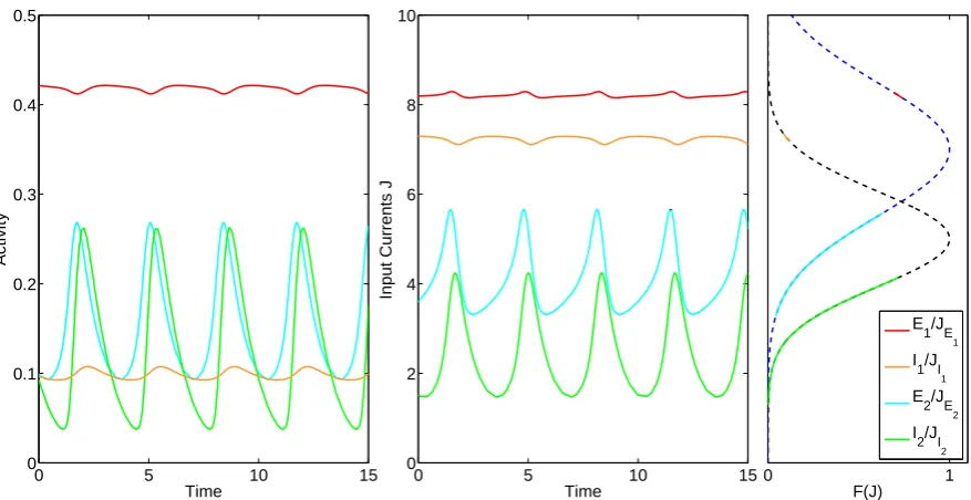
For the linked asymmetric high-low activity stable limit cycle found for both B = 2.45 and

B = 3 a time series is shown in figure 3.7. The figure also shows the input currents into

the subpopulations and their dynamical range on the FRF. For the high activity population the excitatory and inhibitory subpopulation have high and low activity respectively, while for the low population both the excitatory and inhibitory subpopulations have both low activity. The excitatory subpopulations are in anti-phase while the inhibitory subpopulations are in-phase. This is due to the nature of the Gaussian function. If the inhibitory subpopulations receive enough activity to be on the right half of the Gaussian, then extra activity from the excitatory subpopulation is mapped onto a lower firing rate and thus less inhibitory activity. This also happens between the excitatory populations. If both subpopulations have a dynamic range on the left or right half on the Gaussian, they are in-phase or in anti-phase respectively.

This figure also shows why the high activity is stable. Suppose a population has high

excitatory activity, then the inhibitory subpopulations receives a lot of input current sincewEI

is large. This input current is mapped onto a small firing rate and thus the inhibitory activity is and stays small. The excitatory subpopulation then receives a small inhibition current and due to its self-excitation current stays at a high activity level. This high activity equilibrium is thus stable for a single population. Now suppose we receive an extra input current from a neighboring population while the population is in the high activity equilibrium. The current into the population is now larger and mapped onto a lower firing rate and thus the excitatory population becomes less active. This is counteracted by the self-excitation current. Lower activity means less self-excitation and thus the input current becomes smaller. This in turn is mapped on a larger firing rate and thus higher activity. The self-excitation and the neighboring current will balance themselves out and the population will settle on a slightly larger input

current and corresponding lower activity. Indeed, figure 3.6b shows that the high excitatory

activity of the unstable asymmetric equilibrium decreases if the coupling strength becomes larger.

A time series along with its projection on the (E1, E2) of the quasi-periodic solution from

figure 3.6is shown in figure3.8. The time series suggest that the series first stays near the

anti-phase solution, from which it escapes to the in-phase solution for a time and returns back

to the anti-phase solution and so on. Increasingα, we find that the solution disappears via a

−10 −0.5 0 0.5 1 1.5 2 0.1

0.2 0.3 0.4 0.5

Coupling Strength α

Min/Max E

PF 1

PF

3 PF₅

PF 4

PF 2

(A)

−10 −0.5 0 0.5 1 1.5 2

0.1 0.2 0.3 0.4 0.5

B=3; w

EI=18

Coupling Strength α

Min/Max E

PF 2

PF₁

PF 3

PF 4

(B)

Figure 3.6: One parameter diagrams forB = 2.45(top) andB = 3(bottom). Black:

Symmet-ric equilibria; Blue: AsymmetSymmet-ric equilibria; Green: SymmetSymmet-ric Oscillations; Red: AsymmetSymmet-ric Oscillations; Light blue: Antiphase Oscillations; Purple: Quasi-periodic oscillations. For the oscillations only the extrema are indicated. Thick solid and thin dashed lines indicate stable and unstable solutions respectively. At each pitchfork bifurcation (PF) two branches appear of

0 5 10 15 0 0.1 0.2 0.3 0.4 0.5 Time Activity

0 5 10 15

0 2 4 6 8 10 Time

Input Currents J

0 1

F(J) E

1/JE

1 I₁/J_I

1 E₂/J_E

2 I

2/JI

2

Figure 3.7: Left: Time series of the activity of the subpopulations for B = 2.3 and α = 0.1;

Middle: Input currents into each subpopulation; Right: The dynamical range of input currents

J along the excitatory (blue) and inhibitory (black) FRF. Red: E1; Orange: I1; Light blue: E2;

Green: I2. The high and low activity populations resides on the right and left halfs of the

Gaussian FRF respectively.

2000 210 220 230 240 250 260 270 280 290 300

0.05 0.1 0.15 0.2 0.25 0.3 0.35 0.4 Time Excitatory Activity

0 0.05 0.1 0.15 0.2 0.25 0.3 0.35 0.4

0 0.05 0.1 0.15 0.2 0.25 0.3 0.35 0.4 E₁ E2

Figure 3.8: Left: Time series of the activity of excitatory populations of the quasi-periodic

solution for B = 3and α = 0.115. Right: Projection to the (E1, E2)plane. When the torus is

3.3

Multiple populations

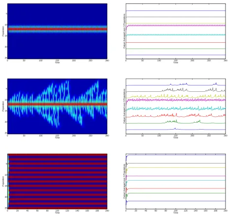
The previous sections showed that due to a Gaussian FRF a new high activity equilibrium ex-ists. This equilibrium in turn forced its neighbor to oscillate as shown in the previous section. Here we use this high activity population as a driver to the whole neural network. All popu-lations start in low activity and we stimulate one population enough to force it into the high excitatory activity stable equilibrium. The stimulated population is chosen such that it is next to

the middle to avoid symmetry in the network. Figure3.9shows the spread of activity through

the network.

For a background currentB= 2.3the populations are located in area 2 in figure3.4where

the low and high activity equilibria are the only invariant sets. The high activity population provides sufficient input current to bring its neighboring populations into area 16, where only a stable limit cycle exists for low activity. These oscillations are not strong enough to force their

neighbors into this area and thus the activity does not spread. If the background currentB =

2.45only a small additional current into a population is needed for it to start oscillating. Thus,

oscillations start to ride on the background input. For large coupling strengthαand largeB, the

network reaches a steady state in which the populations are active in an alternating pattern. This is a direct effect of the Gaussian FRF: Due to symmetry of the function high and low currents are mapped onto a similar firing rate. The high background current forces populations into the high activity stable equilibrium. The high coupling strength in turn forces the high activity populations into a depolarization block. These two mechanisms balance each other out

and results in the alternating pattern. The right side of figure3.9shows the average of the input

currents for the excitatory subpopulations over 3 neighbors. For B = 2.45we see that every

so many cycles three or more populations are activated and start oscillating. These waves end when they reach the boundary or when several populations are active simultaneously as

occurs aroundt= 152ort= 183. For the other two cases the output does not change spatially

over time once stimulation is terminated.

The dynamics shown in 3.9 are a subset of all possible dynamics. Other dynamics such

as the global low or global high activity equilibria correspond to the network being in a resting or highly active state respectively. Bumps in activity can also exist for several populations simultaneously. Each of these bumps drives the system and interactions between expanding

activity generates new dynamics. The ”random” activity pattern found in [22] also exist if a

Gaussian FRF is used, because these dynamics coexist with the extra dynamics incorporated in the WCG network. The transient behavior and local extinction of activity in this pattern is

related to the quasi-periodic solution seen in figure3.8.

Time

Population

0 50 100 150 200 250 300

5

10

15

20

25

0 50 100 150 200 250 300

Time

Output Averaged over 3 Populations

Time

Population

0 50 100 150 200 250 300

5

10

15

20

25

0 50 100 150 200 250 300

Time

Output Averaged over 3 Populations

Time

Population

0 20 40 60 80 100 120 140 160 180 200

5

10

15

20

25

0 20 40 60 80 100 120 140 160 180 200

Time

Output Averaged over 3 Populations

Figure 3.9: Left: Activity of excitatory populations after stimulation between 1 ≤ t ≤ 5 with

parameters {B = 2.3, α = 0.1} (top),{B = 2.45, α = 0.1} (middle) and {B = 3, α = 0.6}

C

HAPTER

4

D

YNAMICS WITH A

P

ROPAGATION

D

ELAY

In this chapter we study the effect of using a propagation delay for activity between populations on the dynamics of a network of Wilson-Cowan populations with a Gaussian firing rate function. The addition of a propagation delay turns the nonlinear WCG differential equations into delay differential equations. With a delay differential equation the derivative of a function depends on the state of the function some time ago, i.e. the history. In this model a fixed delay is used to transfer activity from one excitatory subpopulation to its neighbor(s). In the previous chapter we found different kinds of oscillations. Some of the oscillations only existed when a Gaussian firing rate function was used, such as the driving population and its oscillating neighbors. Other solutions also existed when a sigmoid firing rate function was used, such as the in-phase, anti-phase and quasi-periodic solutions. Depending on the background current and coupling strength between excitatory populations these solutions existed simultaneously with the high-low activity oscillations in the case of two coupled populations.

Here we will look at the existence and region of stability of the periodic solutions in a small network of two coupled populations with a propagation delay. We use the Matlab package

DDE-BIFTOOL [31] to continue the periodic solutions in the time delayτ and coupling strength

α and look at the stability. An analysis on the region of existence and stability is done and is

compared to the system without a propagation delay.

Continuing the structure in the previous chapter we look at a large network of populations with a propagation delay. Simulations are made to link the results of the network of two coupled populations to this larger network. Different types of activity patterns are shown and classified.

A classification diagram is made to show which dynamics are most prevalent for pairs ofτ and

α.

4.1

Two coupled populations

Here we look at two coupled populations with a propagation delay for transfering activity. Look-ing at the case without a propagation delay we find in-phase (IP), anti-phase (AP), a-periodic and high-low (HL) activity oscillations. Each of these oscillations exists in a certain parameter

range of background currentB and coupling strengthα. In accordance to the structure of the

previous chapter we determine the region of stability in two cases: B = 2.45 andB = 3. The

region of stability is a subset of the region of existence. By simulating two populations, using

dde23in Matlab, we look for the periodic solutions for certainτ and α. In this study we chose

to to scan the(τ, α)-space along 32 lines for τ = k₄ with k= 0...32 and look at the stability of

each computed point. Figure4.1shows the bounds in which the periodic solutions are stable

forB = 2.45andB= 3.

Case A

ForB = 2.45the HL solution is stable for allτ ∈[0,8]. The upper bound forαchanges withτ

and the period is around 2. Ifαbecomes too large the low activity population receives enough

upper bound forαin which the solution is stable is related to the period. The upperbound is at

its maximum if the solution is in anti-phase a time lengthτ ago. Because the resolution of the

grid is poor this is only roughly true for the peaks in the figure. The upper bound converges

to α ≈ 0.25 if τ becomes large. The lower bound forα = 0.028comes from the homoclinic

bifurcation and is also found in the case without a propagation delay. If the coupling strength is too small, the high activity population does not provide enough current for the low activity population to cross the bifurcation curve. The delay does not matter because the high activity equilibrium is stable without extra current from its neighbor. The AP solution is not stable for

τ < 0.4. Forτ ∈ [0.4,6.8]the lower and upper bounds of alpha show where the solution is

stable. Atα = 0.4 andα = 6.8the periodic solution vanishes due to a homoclinic bifurcation.

The IP solution does not exist forB = 2.45. The figure can be found in figure4.1a.

Case B

For B = 3 the HL solution is stable. The existence does not depend on τ, but the stability

boundary strongly onα. On the upper bound the period of the solution is around2. The time

delay between two peaks of the upper bound for alpha is approximately1.5. The lower bound

is smaller than zero and is not shown. The AP solution is stable forτ > 0 depending on the

value of α. The upper bound also slowly oscillates. At τ = 1 the solution becomes stable

for certain values of α. The region of stability for the IP solution looks similar to the region

of the AP solution, but shifted to the right. A time delay of half a period corresponds to an input current of an anti-phase solution and explains their similarity . The lower bounds for the solutions are smaller than zero and not shown. Simulations, starting from random low activity history, show that the anti-phase and in-phase region of attractions change when the delay changes. Simulations for a certain parameter pair always go to either the anti-phase or the

in-phase solution for lowα. For intermediateαthe quasi-periodic solution becomes dominant,

while for largeα the populations either go to the high-low periodic solution or the symmetric

high activity equilibrium. The figure can be found in figure4.1b.

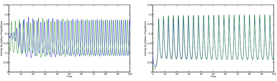
Figure4.2shows the in-phase and anti-phase periodic solution. The activities are constant

for the history t ∈ [−τ,0]and are chosen randomly with Ek, Ik ∈ [0,0.25];k = 1,2. The time

series converges to the in-phase or anti-phase solutions. For these parameter values the region of attraction of the anti-phase solution is much larger. This is one of the few regions in which solutions for both the anti-phase as in-phase solutions could be found.

0 1 2 3 4 5 6 7 0

0.1 0.2 0.3 0.4 0.5

Time Delay τ

Coupling Strength

α

(A)

0 1 2 3 4 5 6 7

0 0.1 0.2 0.3 0.4 0.5

Time Delay τ

Coupling Strength

α

(B)

Figure 4.1: The lines indicate the upper and lower bounds in between which the periodic

solutions are stable withB = 2.45(left) andB = 3(right). Stability was calculated atτ = 0.25k

withk = 0...32 and lines were drawn between the points. The dashed lines in the right figure

are the upper bound in which simulations showed in-phase or anti-phase solutions. IfB = 3the

lower bounds are smaller than zero and not shown. Note that the solid and dashed lines only

overlap forτ <2. Red: High-low activity; Green: In-phase low activity; Light blue: Anti-phase

low activity.

0 10 20 30 40 50 60 70 80 90 100

0 0.05 0.1 0.15 0.2 0.25 0.3 0.35

Time

Activity Excitatory Populations

0 10 20 30 40 50 60 70 80 90 100

0 0.05 0.1 0.15 0.2 0.25 0.3 0.35

Time

Activity Excitatory Populations

Figure 4.2: Time series for the anti-phase (left) and in-phase (right) solutions forα= 0.05, τ = 4

Time Delay τ

Coupling Strength

α

0 0.2 0.4 0.6 0.8 1 1.2 1.4 1.6 1.8 2

0.17 0.16 0.15 0.14 0.13 0.12 0.11 0.1 0.09 0.08 0.07 0.06

Time Delay τ

Coupling Strength

α

2.5 3 3.5 4 4.5 5 5.5 6 6.5 7 7.5

0.17 0.16 0.15 0.14 0.13 0.12 0.11 0.10 0.09 0.08 0.07 0.06

Figure 4.3: Classification of patterns after starting from random low activity history for various

τ and α. Left: Small time delay; Right: Large delay. The figure on the left shows that

quasi-periodic and bump activity disappears for a medium delay. The right figure shows that the in-phase solution becomes stable for a large delay. Dark blue: Low stable equilibrium; Yellow: Quasi-periodic; Light blue: Anti-phase; Green: In-phase; Red: Local bump in activity; Dark Red: High activity for all populations.

4.2

Multiple populations

The regions of stability found in the two populations do not directly transfer over to a network

with multiple (> 2) populations, since in a larger network a population receives input current

from two neighboring populations. An analytic approach to analyzing this network is outside the scope of this study, due to the computational requirements needed for all the computations.

Instead we classify patterns and record their appearance for a range of values ofαandτ.

We simulate 25 connected populations with the boundary populations connected to each other, thus the network forms a circle. Each population starts with random low activity history

(Ek(t), Ik(t) ∈ [0,0.25] fort ∈ [−τ,0] with k = 1...25). For each {τ, α} pair 4 simulations are

made and each pair is classified according to the most prevalent dynamics. For the

classifica-tion we looked at the state the network was in fort∈[100,200]. In the case that certain activity

patterns coexist more simulations were done to determine a dominant pattern. Nonetheless this classification method only gives a qualitative estimate for certain patterns to appear.

In figure 4.3 we show the classification for each{τ, α} pair. We distinguish between the

patterns found in figure4.4in addition to the global low and high activity equilibria. For a small

time delayτ <0.6we see that the quasi-periodic and activity bump pattern are prevalent for low

and highαrespectively. Aroundτ = 0.6we see that the anti-phase pattern becomes dominant

for mediumα. If we increaseτ further we see that the global high activity equilibrium becomes

more dominant for a larger rangeαat the expense of the anti-phase pattern. The classification

does not change much until we reachτ = 4where the in-phase solution becomes common in

the simulations for a small range ofα.

Figure 4.4shows the patterns the can appear for variousτ andα in addition to the global

low and high activity equilibria. Figure 4.4ashows local bumps in activity. These bumps are

stable and drive the system and can be linked to the HL periodic solution in the two

popu-lation case. Figures 4.4b and 4.4c show the anti-phase and in-phase pattern. Their period

increases with the time delay. The more chaotic pattern in the figure 4.4d could come from

the quasi-periodic solution found in the analysis of two population without delay. We see that if populations synchronize locally activity extinguishes. Examples of this synchronization can be

Time

Population

0 20 40 60 80 100 120 140 160 180 200

5

10

15

20

25

Time

Population

0 20 40 60 80 100 120 140 160 180 200

5

10

15

20

25

Time

Population

0 20 40 60 80 100 120 140 160 180 200

5

10

15

20

25

Time

Population

0 20 40 60 80 100 120 140 160 180 200

5

10

15

20

25

Figure 4.4: Different patterns in a neural network for (a){α= 0.15, τ = 0.2}, (b){α= 0.12, τ =

C

HAPTER

5

D

ISCUSSION

In this study we have investigated the dynamics of a neural network governed by the Wilson-Cowan equations. In particular, we have chosen a Gaussian firing rate function, rather than the default sigmoid. Also, a propagation delay between the excitatory subpopulations was added. Some of the attractors we found using bifurcation analysis have been found in earlier studies for the case with zero propagation delay. When a Gaussian shaped firing function is used, an additional high activity is shown to exist. With multiple coupled populations this high activity population provided enough drive for surrounding populations to start oscillating. For certain parameter ranges one driving population could spread activity throughout the whole network.

The Gaussian firing rate function was motivated by observations of ictal activity using a Utah array. An experimental firing rate function could be determined using the low-frequency component of the local field potential to represent synaptic input, and the high-frequency com-ponent as spike output. For some cases this showed a nonmonotone relationship suggesting the choice for the Gaussian function. The experimental curve with low-frequency local field potential (L-LFP) plotted versus the high frequency components as a firing rate index suggests that beyond the maximum a plateau is reached, not unlike a depolarization block. For sim-plicity we have modeled the firing rate function as a Gaussian such that it returns to zero for high input current. With a certain set of parameter values, chosen such that the influence of the Gaussian FRF became most clear, an additional equilibrium with high excitatory and low inhibitory activity was found. This equilibrium coexists with the usual dynamics found in the sigmoid case. In this high activity equilibrium the inhibitory population receives enough input current and the inhibitory firing rate is low due to the shape of the FRF. This inhibitory firing rate is low enough for the excitatory population to receive low inhibition and thus remain highly active. This behavior of the inhibitory subpopulation could be seen as a depolarization block on a neural mass level. Due to the Gaussian shape the activity and input current vary much. Oscillating high activity populations receive an large input current with low amplitude, while its oscillating neighbors receive a relatively small input current with large amplitude.

The dynamic range of the excitatory firing rate function was just after the peak in the sian, not unlike the experimental curve. The nullclines of a single E-I pair show that the Gaus-sian shape of the inhibitory subpopulation is more important than the shape of the excitatory subpopulation. A sigmoid firing function for the excitatory population would probably suffice to create similar dynamics, since the shape of the nullcline is not qualitatively different from the Gaussian one in the used domain.

The bifurcation analysis for two coupled local populations without propagation delay showed multiple stable attractors. In-phase, anti-phase and quasi-periodic periodic solutions have been

found around a low steady state, their existence depending on the coupling strengthα. These

We explored with a propagation delay between the excitatory the subpopulations region of stability for periodic solutions. The in-phase low activity solution became stable if a large propagation delay was added for small background currents. The stability region of the linked high and low activity oscillations resonated with the period of the oscillations. The existence of these oscillations depend only the coupling strength and not on the delay. The stability of each periodic solution is computed on a low resolution grid and thus results are not exact. Also no differentiation has been made between the different kind of bifurcations these periodic solutions have. Simulations showed that the region of attraction of the in-phase and anti-phase changed with the delay. The quasi-periodic attractor has a large region of attraction for parameter ranges in which both the in-phase as anti-phase solutions are stable.

For larger networks with propagation delay, a link was created between the time delay, cou-pling strength and the different kinds of stable patterns. With a small delay the quasi-periodic and local bumps in activity are the dominant patterns. For intermediate coupling strength and intermediate or high propagation delay the low activity anti-phase solution is the most domi-nant. Although the in-phase solution is stable, the anti-phase solution has a larger region of attraction for all but a few parameter ranges. Considering this, the effect of a propagation delay is important for the region of attractions in neural networks. The quasi- periodic solution for intermediate coupling strength exists in both the sigmoid as in the Gaussian case. The nature of this solution could explain the ”random” times local extinction of activity occurs, since the solution skirts close to the in-phase solution, in which case the activity dies out locally if the background input is small. A further study of the nature of this solution could be done.

Epilepsy is characterized by transitions between normal and ictal activity. Although for certain parameter ranges our model produces transient activity, as with the quasi-periodic so-lutions, in general the model does not provide internal means to switch between those states. The different patterns found in the larger network are very stable and transitions between them are rare. Global parameter transitions however, could force a switch between

differ-ent states. Infludiffer-ential parameters are the background currdiffer-ent B, local connectivity wEI and

coupling strength α. Local or global stimulation patterns, adaptation and synaptic plasticity

between subpopulations or populations could force transitions between states through new dynamics.

The actual micro-electrode array used in the experiments uses a 2D grid with electrodes. In our model however, we use a 1D grid. A study using the sigmoid firing rate function showed

some possible dynamics of the network [22]. Here an external oscillation introduced to the

center population formed waves of activity. With a Gaussian function a driving population instead could produce waves of activity throughout the system.

R

EFERENCES

[1] R. S. Fisher, W. Van Emde Boas, W. Blume, C. Elger, P. Genton, P. Lee, and J. Engel Jr., “Epileptic seizures and epilepsy: Definitions proposed by the international league against

epilepsy (ilae) and the international bureau for epilepsy (ibe),” Epilepsia, vol. 46, no. 4,

pp. 470–472, 2005.

[2] F. H. L. Da Silva, J. A. Gorter, and W. J. Wadman, Epilepsy as a dynamic disease of

neuronal networks, vol. 107 ofHandbook of Clinical Neurology. 2012.

[3] R. FitzHugh, “Impulses and physiological states in theoretical models of nerve

mem-brane,”Biophysical Journal, vol. 1, no. 6, pp. 445 – 466, 1961.

[4] N. Fourcaud-Trocm ´e, D. Hansel, C. Van Vreeswijk, and N. Brunel, “How spike

genera-tion mechanisms determine the neuronal response to fluctuating inputs,” The Journal of

neuroscience, vol. 23, no. 37, pp. 11628–11640, 2003.

[5] A. L. Hodgkin and A. F. Huxley, “A quantitative description of membrane current and its

application to conduction and excitation in nerve.,” The Journal of physiology, vol. 117,

no. 4, pp. 500–544, 1952.

[6] N. F. Rulkov, “Modeling of spiking-bursting neural behavior using two-dimensional map,”

Phys. Rev. E, vol. 65, p. 041922, Apr 2002.

[7] E. M. Izhikevich,Dynamical systems in neuroscience. MIT press, 2007.

[8] J. Rinzel, “Discussion: Electrical excitability of cells, theory and experiment: Review of

the hodgkin-huxley foundation and an update,” Bulletin of Mathematical Biology, vol. 52,

no. 1, pp. 5–23, 1990.

[9] H. R. Wilson and J. D. Cowan, “Excitatory and inhibitory interactions in localized

popula-tions of model neurons,”Biophysical journal, vol. 12, no. 1, pp. 1–24, 1972.

[10] H. R. Wilson and J. D. Cowan, “A mathematical theory of the functional dynamics of

cortical and thalamic nervous tissue,”Kybernetik, vol. 13, no. 2, pp. 55–80, 1973.

[11] F. H. Lopes da Silva, A. Hoeks, H. Smits, and L. H. Zetterberg, “Model of brain rhythmic

activity. the alpha rhythm of the thalamus,”Kybernetik, vol. 15, no. 1, pp. 27–37, 1974.

[12] B. H. Jansen, G. Zouridakis, and M. E. Brandt, “A neurophysiologically-based

mathe-matical model of flash visual evoked potentials,” Biological cybernetics, vol. 68, no. 3,

pp. 275–283, 1993.

[13] F. Wendling, F. Bartolomei, J. J. Bellanger, and P. Chauvel, “Epileptic fast activity can

be explained by a model of impaired gabaergic dendritic inhibition,” European Journal of

Neuroscience, vol. 15, no. 9, pp. 1499–1508, 2002.

[14] S.-I. Amari, “Homogeneous nets of neuron-like elements,”Biological Cybernetics, vol. 17,

no. 4, pp. 211–220, 1975.

[15] A. Destexhe and T. J. Sejnowski, “The wilson–cowan model, 36 years later,” Biological cybernetics, vol. 101, no. 1, pp. 1–2, 2009.

[16] R. M. Borisyuk and A. B. Kirillov, “Bifurcation analysis of a neural network model,”

Biolog-ical Cybernetics, vol. 66, no. 4, pp. 319–325, 1992.

[17] A. C. Marreiros, S. J. Kiebel, and K. J. Friston, “A dynamic causal model study of neuronal

population dynamics,”Neuroimage, vol. 51, no. 1, pp. 91–101, 2010.

[18] A. Borisyuk and J. Rinzel, “Understanding neuronal dynamics by geometrical dissection

of minimal models,” Methods and Models in Neurophysics, Proceedings of Les Houches

Summer School Elsevier, pp. 19–72, 2005.

[19] P. Bressloff and S. Coombes, “Physics of the extended neuron,” International Journal of

Modern Physics B, vol. 11, no. 20, pp. 2343–2392, 1997.

[20] C. A. Schevon, S. A. Weiss, G. McKhann Jr, R. R. Goodman, R. Yuste, R. G. Emerson, and A. J. Trevelyan, “Evidence of an inhibitory restraint of seizure activity in humans,”

Nature communications, vol. 3, p. 1060, 2012.

[21] G. N. Borisyuk, R. M. Borisyuk, A. I. Khibnik, and D. Roose, “Dynamics and bifurcations

of two coupled neural oscillators with different connection types,”Bulletin of mathematical

biology, vol. 57, no. 6, pp. 809–840, 1995.

[22] R. Borisyuk and Y. Kazanovich, “Oscillations and waves in the models of interactive neural

populations,”Biosystems, vol. 86, no. 1, pp. 53–62, 2006.

[23] M. Goodfellow, K. Schindler, and G. Baier, “Intermittent spike-wave dynamics in a

hetero-geneous, spatially extended neural mass model,” NeuroImage, vol. 55, no. 3, pp. 920–

932, 2011.

[24] S. Coombes and C. Laing, “Delays in activity-based neural networks,” Philosophical

Transactions of the Royal Society A: Mathematical, Physical and Engineering Sciences, vol. 367, no. 1891, pp. 1117–1129, 2009.

[25] A. Hutt and F. M. Atay, “Effects of distributed transmission speeds on propagating activity

in neural populations,”Physical Review E, vol. 73, no. 2, p. 021906, 2006.

[26] A. Roxin and E. Montbri ´o, “How effective delays shape oscillatory dynamics in neuronal

networks,”Physica D: Nonlinear Phenomena, vol. 240, no. 3, pp. 323–345, 2011.

[27] S. A. Campbell, “Time delays in neural systems,” in Handbook of brain connectivity,

pp. 65–90, Springer, 2007.

[28] Y. Kuznetsov,Elements of Applied Bifurcation Theory, vol. 112. Springer, 2004.

[29] A. Dhooge, W. Govaerts, Y. A. Kuznetsov, H. Meijer, and B. Sautois, “New features of

the software matcont for bifurcation analysis of dynamical systems,” Mathematical and

Computer Modelling of Dynamical Systems, vol. 14, no. 2, pp. 147–175, 2008.

[30] J. Polking,Ordinary Differential Equations Using MATLAB. Pearson/Prentice Hall, 2004.

[31] K. Engelborghs, T. Luzyanina, and G. Samaey, “Dde-biftool v. 2.00: a matlab package for