Cyclic gravity waves in deep water

CYCLIC GRAVITY WAVES IN DEEP WATER

by

P. J. Bryant

P.J. BRYANT

ABSTRACT

Numerical evidence is presented for the existence of unsteady periodic gravity waves of large height in deep water whose shape changes cyclically as they propagate. It is found that, for a given wavelength and maximum wave height, cyclic waves with a range of cyclic periods exist , with a steady wave of permanent shape being an extreme member of the range. The method of solu-tion, using Fourier transforms of the nonlinear surface boundary conditions, determines the irrotational velocity field in the water and the water surface displacement as functions of space and time, from which properties of the waves are demonstrated. In particular, it is shown that cyclic waves are closer to the point of wave breaking than are steady permanent waves of the same wave height and wavelength.

1. INTRODUCTION

This investigation began with the development of a numerical method for obtaining periodic wave group solutions of permanent envelope in which neither the small wave height nor the narrow wave-band assumptions were made. Solutions were calculated as the

envelope length to wavelength ratio was decreased step by step until the two lengths were equal. It was discovered then that solutions with the two lengths equal still existed as the envelope velocity was increased step by step. This set of periodic wave group solutions, with the envelope length equal to the wavelength, and with a range of envelope velocities, is the subject of the present investigation.

It is simpler to interpret these waves in a frame of reference moving with the wave velocity rather than with the envelope velocity. Relative to the wave velocity, the shape of the wave train changes cyclically as it propagates, as though it we~e a periodic wave train set into an oscillation about a permanent shape. If this

inter-pretation is accepted, it is reasonable also to accept that there should be a range of periods of shape oscillation, dependent on the amplitude of the shape oscillation, because the phenomenon is non-linear. The range of periods of shape oscillation in the wave

interpretation is equivalent to a range of envelope velocities in the envelope interpretation. Although the numerical calculations were made relative to a frame of reference moving with the envelope velocity, they are presented here in terms of the wave interpretation.

2. THEORY

<Pxx + <Pyy

=

O Y < sn(x,t) I ( 2. la)

<Px,<Py-+ 0 as

nt - <Py+ snx<Px

1 2

n + <Pt +

2

s (<j)x

y-+-CO

O I

(2. lb)

y

=

sn(x,t), (2. le)

= 0 , y = sn(x,t). (2.ld)

The dimensional variables are the surface displacement an, the

~ ~

velocity potential (g,Q,) a¢ , and ix, Q,y, (Q,/g) t . Symmetric permanent wave solutions exist for which

n

=

~ ak cos{k(x - ct)} , <P = k b eky sin{k(x - ct)}

k k

The nonlinear algebraic equations for the first 2N amplitudes

(2. 2a) (2. 2b)

ak, bk, k = 1,2, ..• N and the velocity c, .obtained by substituting the terminated series for

n

and <Pinto equations (2.lc,d), may be solved numerically for a given value of€ by one of a number of methods. For instance, the 2N + 1 variables may be found by solving the 2N boundary conditions (2.lc,d) at each of N equally spaced points over a half-wavelength O < x - ct< TI, together with the kinematic equation

n

=

1 at x - ct= 0. This in essence is the

method used by Rienecker and Fenton [2]. Alternatively, for a better description of the wave crest at large wave heights, the N points may be equally spaced in they-direction over the above half-wavelength, using successive approximations to achieve this spacing. A third methotl is to take Fourier transforms of the boundary

conditions (2.lc,d) after the terminated series for

n

and <P have been substituted, and to put each of the Fourier coefficients to zero to find numerically ak, bk, k = 1,2, ... N, and c. This is the method used in the present investigation.

Y)

= L

:1: a

k jk cos{k (x - ct) + jat}

'

(2. 3a) j

¢

= LL

_{bjk eky sin{k (x - ct)} + jat}

.

(2. 3b)

j k

The wave velocity is c in the sense that, relative to a frame of reference moving with velocity c, the wave shape oscillates with an angular frequency

a

about a symmetric shape. The terminated series for Y) and¢ are substituted into the boundary conditions (2.lc,d) and double Fourier transforms with respect to x - ct and tare calculated numerically. Each of the Fourier coefficients is put to zero to calculate numerically a finite number of amplitudes ajk' bjk and the frequency

a

for given values of E and c.

Before expanding the method in more detail, the amplitudes

ajk' bjk are discussed as functions of j and k. Each j is regarded as defining a waveband containing all harmonics with

wavenumbers k;;;,, O, and amplitudes ajk' bjk for the given value of j. The dominant waveband j = O, containing amplitudes

aOk' bOk' k

=

1,2, .•. , describes the time independent contribution to the cyclic wave in a frame of reference moving with the wave velocity. The amplitude a

00 is zero because Y) has a zero mean, and the amplitude b

00 is zero since any other value in the expansion (2.3b) is meaningless. The waveband j

=

1 contains amplitudes

alk' k

=

1,2, ... , and blk' k

=

0,1,2, •.. , with a₁₀ being equal to zero because Y) has a zero mean. The waveband j = - 1 contains

amplitudes a-l,k' k

=

1,2, ... , and b-l,k' k

=

1,2, •.. , since b_

110 is included with b10. Similarly, successive wavebands j 2,3, ... and j = -2,-3, ... each contain amplitudes ajk' bjk' k 1,2, ... together with bjO when j > O. The trend of the magnitudes of the amplitudes is towards zero as jj

I

and k increase,

The series (2.3a,b) are substituted now into the boundary conditions (2.lc,d) with. the abbreviations

c jk = cos {k (x - ct) + jat}

sjk sin {k (x - ct) + jat}

If the resulting expressions are denoted by F and G, then

F = I: I: { (kc - ja) a 'ks 'k - kb 'keskns .k}

j k J J J J

- s(I: I: ka.ks.kJ x

(1:

I: kb.kesknc.k) =

o ,

(2.4a)

j k J J j k J J

G = I:

L

{a .kc 'k - (kc - ja) b .ke sknc .k}

j k J J J J

+ _21 s

(L

L kb 'kesknc .kJ z + ~21 s

[L

L kb 'kei::kns 'k) z =

o ,

j k J J j k J J

(2.4b) where eskn

=

exp{sk

LL

a c } . The definition of E: is equivalent

p q pq pq to

H

= L L

a = 1 .

j k jk

Equations (2.4a,b) may be transformed numerically to

F = LL F s 0 m n mn mn G = LL G c 0

mn mn

_'

m n

from which

F = G = 0 , all m,n .

rnn mn

(2.4c)

(2. Sa)

(2. Sb)

(2. 6)

The Fourier coefficients Fmn, Gmn are nonlinear functions of ajk' bjk and Cl. Equations (2.6) may be solved numerically by Newton's

method, which for Fis described by

L L ['\ 8F

J

(a 'k - a '.k) + L L ['\bdF

J

(b 'k - b '.k) +

j k oajk mn J J j k a jk mn J J

(dF]

aa

rnn ( Cl - Cl ) 1 = F mn ' ( 2. 7)

m,n Fourier coefficient of a partial derivative of equation (2.4a),

and the prime denotes the new value of each variable. The coefficients and the right of equation (2.7) are evaluated at the old values of

the variables. There is a similar set of equations derived from G and a single equation derived from H. The complete set of linear

I

equations is solved numerically for the differences ajk - ajk' bjk - bjk' a - a', the new values of the variables are calculated, and the process is repeated until the differences are less than some small arbitrary number (l0-10 in the examples following).

The range of solutions was explored as the amplitude ratios and the wave velocity c were changed step by step. In general, the method converged to the cyclic wave solutions without difficulty, the only exception being for cyclic wave solutions near to permanent wave solutions, when care had to be taken to keep the solution

converging on the right path. One advantage of the Fourier transform method is that the Fourier coefficients F , G may be found for

mn mn

wavebands m and wavenumbers n outside those included in the calculation. This information then shows which wavebands and which wavenumbers

should be included in the calculation to improve the precision with which equations (2.Sa,b) are satisfied over the complete range of

x and t.

3. EXAMPLES

A range of cyclic wave solutions exists for certain given

Each range of solutions had a lower bound as c was decreased at given €, but it has not been possible to isolate the physical constraint which determines this lower bound. No cyclic wave solutions could

be found for€ less than 0.261, when the wave height to wavelength ratio is 0.0737 as the cyclic wave passes through its maximum height and the cyclic wave is almost a permanent wave. It appears that cyclic waves on deep water exist only at wave height to wavelength ratios which are more than one half of the maximum wave height to wavelength ratio for steady waves of permanent shape on deep water.

Although the range of solutions could be explored with equations (2.Sa,b) satisfied to low precision with few harmonics, computer restrictions meant that only a few examples could be calculated to high precision with many harmonics. Four such examples are presented below, with the second, third and fourth examples containing as many harmonics as could be manipulated in double precision by a Prime 750 computer.

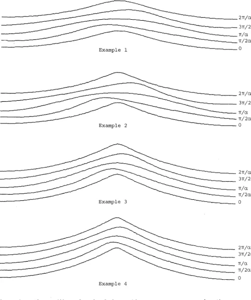
The profiles of the four cyclic wave solutions over one wave-length and one cycle of shape, relative to a frame of reference moving with the wave velocity, are sketched in figure 1. Starting from the symmetric initial shape, the crest moves backwards, then forwards through the centre, and finally back to the centre. noted, from equation (2.3a), that

n(x- ct,t) = n(2TI- (x- ct), 2TI/a- t).

It is

(3 .1)

The symmetric shape in the middle of the cycle (t = TI/a) is flatter than that at the ends of the cycle (t

=

O, 2TI/a). The data for the examples are now summarised.

Example 1

s

=

0.3,

c

=

1.0273, a= 0.5273

The wave height to wavelength ratio at maximum wave height in the

cycle is 0.0757 with a particle velocity at the crest of 0.3749 at this instant. The final solution contains 217 harmonics (435

variables) in 14 wavebands - 3

<

j

<

10, the wavenumber range being The maximum Fourier coefficient F . , G not included

mn mn

has magnitude 5 x 10-7• The maximum magnitude of F and Gover the

64 x 64 points in space and time used for the final calculation is

3.8 x 10-5 with a root mean square deviation from zero of 1.8 x 10-5•

Those harmonics with amplitudes greater than 10-s in magnitude are tabulated in the Appendix. (A computer listing of all harmonics calculated for this and the following examples may be obtained from the author. )

Example 2 s = 0.4, c = 1.0404, a= o.4904

The wave height to wavelength ratio at maximum wave height in the cycle is 0.0953 with a particle velocity at the crest of 0.5637

at this instant. The final solution contains 301 harmonics (603

variables) in 17 wavebands - 3

<

j

<

13, the wavenumber range being

0

<

k

<

31. The maximum Fourier coefficient F , G not included

mn mn

has magnitude 5.2 x 10-5• The maximum magnitude of F and Gover

the 64 x 64 points in space and time used for the final calculation

is 3.6 x 10-3 with a root mean square deviation from zero of

2.6 x 10-4•

Example 3

s

=

o.5,

c

=

1.0672, a= 0.3972

The wave height to wavelength ratio at maximum wave height in the cycle is 0.1215 with a particle velocity at the crest of 0.7188

at this instant. The final solution contains 295 harmonics (591

being O

<

k

<

34. The maximum Fourier coefficient F , G among

mn mn

-4

those not included in the final calculation has magnitude 1.0 x 10 . The maximum magnitude of F and Gover the i28 x 64 points in space

-2

and time is 3.05 x 10 with a root mean square deviation from zero

-3

of 1.5 x 10 (The calculation of the final solution from the

previous solution containing 39 fewer harmonics took about 24 hours of central processor time on a Prime 750 computer.)

Example 4

s

= 0.55,

c

= 1.0799,

a=

0.3199

The wave height to wavelength ratio at maximum wave height in the cycle is 0.1319 with a particle velocity at the crest of 0.8303

at this instant. The final solution contains 303 harmonics (607 variables) in 13 wavebands - 3

<

j

<

9, the wavenumber range being 0

<

k

<

30. The maximum Fourier coefficient F , G among those

mn mn

-4

not included in the final calculation has magnitude 8.2 x 10 The maximum magnitude of F and Gover the 64 x 64 points in space

-2

and time used for the final calculation is 5.2 x 10 with a root

-3

mean square deviation from zero of 3.2 x 10 . The wave profiles and the properties described below were plotted both for the final solution and for the previous solution containing 28 harmonics less, when the only discernible difference was a slight sharpening of the crest in the final solution. Even though it would be preferable to include more harmonics, it does appear that the properties are accurate to within the precision with which the figures are drawn.

It is of interest to compare each of the cyclic wave examples with a corresponding permanent wave example, in particular the

being greater than the wave velocity of the corresponding cyclic wave. The particle velocities at the crests of the four permanent waves are 0.3068, 0.4198, 0.6237, 0.7509, each being less than the particle

velocity of the corresponding cyclic wave. The ratio of the maximum particle velocity at the wave crest to the wave velocity for the

cyclic waves is 0.365, 0.542, 0.674, 0.769 and for the permanent waves is 0.298, 0.401, 0.580, 0.690 respectively. Given the non-uniform properties that have been found for permanent waves as the limiting wave is approached, any extrapolation of properties from large wave heights to the limiting wave height must be treated with caution. However, the trends in the two sets of ratios above suggest that the ratio for cyclic waves may reach one before the limiting wave is reached, after which breaking would occur as a spilling of the

wave crest.

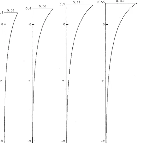
The water motion associated with cyclic waves is examined now

from both the Eulerian and Lagrangian viewpoints. The horizontal velocity profile under a wave crest at the beginning of each cycle is sketched in figure 2 for each of the four examples of cyclic waves.

FIGURE 2 NEAR HERE

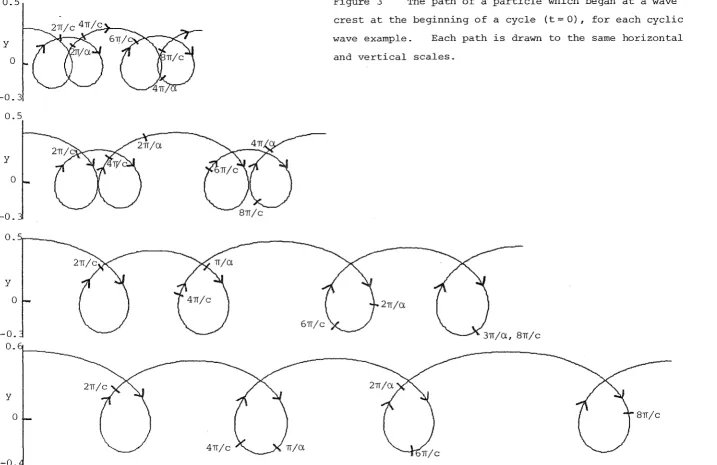
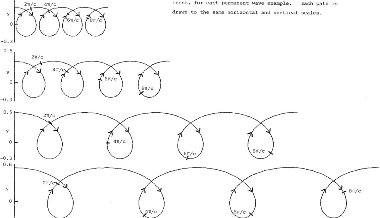
An alternative view of the water motion is provided by the paths

followed by marked fluid particles. The path of a particle which

began at a wave crest at the beginning of a cycle is sketched in

figure 3 for each of the cyclic wave examples, and in figure 4 for

FIGURES 3 AND 4 NEAR HERE

each of the permanent wave examples. The location of the particle

at later times is marked on each path, where 2TI/c is the wave period

and 2TI/a is the period of one cycle of wave shape. (A second order

Runge-Kutta method was used to calculate the particle paths, whose

accuracy could be checked by confirming that the particle remained

on the water surface.) The main difference between the pairs of

particle paths is that the cyclic wave particle paths do not have

any spatial periodicity, since the shape period 2TI/a is not a rational

multiple of the wave period 2TI/c. The net horizontal distance

covered by a fluid particle between loops on its path is less for

the cyclic waves than for the permanent waves, the reason being that

the wave height and hence fluid velocity of the cyclic waves is less

in the middle of a cycle (t

=

TI/a) than at the ends (t

=

0, 2TI/a),

while the height of the permanent waves remains constant. In the

first two examples of cyclic waves, the interval between the first

and second loops lies in the middle of a cycle, making i t shorter

than the interval between the second and third loops which lies at

the end of a cycle.

4. DISCUSSION

The cyclic waves investigated here are particular unsteady

solutions of the equations governing waves on deep water in

(equations 2.3) is a simple unsteady generalisation of the form for single crested permanent waves (equations 2.2). It can be expected that a suitable form of solution describing a two-wavelength wave group can be found which is an unsteady

general-isation of the form for double-crested permanent waves. This in

turn should be capable of further generalisation to all multi-crested permanent waves of the type described by Saffman [ 3].

Ocean waves of large height are modelled often by steady waves of permanent form. It may be more realistic to model regular ocean waves of large height by cyclic waves, since

naturally occurring waves are never completely steady. Longuet-Higgins [ l] derived a number of properties of steady permanent waves near the point of wave breaking, including the existence of a sharp shear at the free surface of a steady wave of maximum steepness. The trend in the cyclic wave examples above, together

with the large increase in high wavenumber harmonics in the velocity field as the wave height approaches the limiting case, suggests that a sharp shear may occur at the free surface of cyclic waves before maximum steepness is reached. Although no difficulties can be

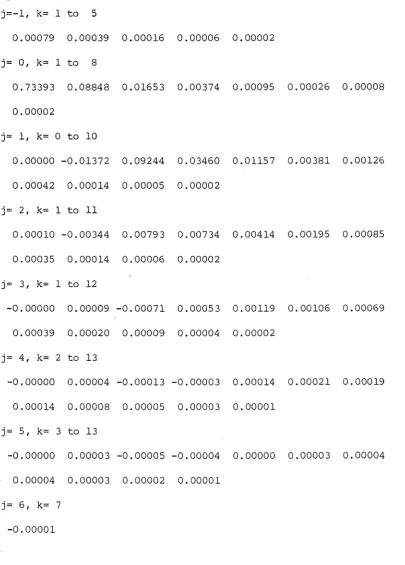
APPENDIX

Table of harmonics for example l with magnitudes exceeding 10 -5

ajk

j=-1, k= l to 5

0.00079 0.00039 0.00016 0.00006 0.00002

j=

o,

k= l to 8

0.73393 0.08848 0.01653 0.00374 0.00095 0.00026 0.00008

0.00002

j= 1, k= 0 to 10

0.00000 -0 .01372 0,09244 0.03460 0 .01157 0.00381 0.00126

0.00042 0. 00014 0.00005 0.00002

j= 2, k= l to 11

0.00010 -0.00344 0.00793 0.00734 0. 00414 0. 00195 0.00085

0.00035 0. 00014 0.00006 0.00002

j= 3, k= l to 12

-0.00000 0.00009 -0. 00071 0.00053 0. 00119 0.00106 0.00069

0.00039 0.00020 0.00009 0.00004 0.00002

j= 4, k= 2 to 13

-0.00000 0.00004 .:..0.00013 -0.00003 0 .00014 0.00021 0. 00019

0.00014 0.00008 0.00005 0.00003 0.00001

j= 5, k= 3 to 13

-0.00000 0.00003 -0.00005 -0.00004 0.00000 0.00003 0.00004

0.00004 0.00003 0.00002 0.00001

j= 6, k= 7

[image:14.595.77.483.143.709.2]

bjk

j=-1, k= l to 5

o.

00077 0.00015 0.00002 0.00000 0.00000

j=

o,

k= l to 8

o.

72784 0.00516 0.00034 0.00003 0.00000 0.00000 0.00000

0.00000

j= 1, k= 0 to 10

-0.00005 -0.03296 0.06498 0.00200 0.00018 0.00002 0.00000

0.00000 0.00000 0.00000 0.00000

::

j=2 I k=l to 11

0.00071 -0.00454 0.00499 0.00045 0.00006 0.00001 0.00000

0.00000 0.00000 0.00000 0.00000

j= 3, k= l to 12

-0.00001 0.00024 -0.00068 0.00045 0.00008 0.00001 0.00000

0.00000 0.00000 0.00000 0.00000 0.00000

j= 4, k= 2 to 13

-0.00001 0.00007 -0.00010 0.00004 0.00001 0.00000 0.00000

0.00000 0.00000 0.00000 0.00000 0.00000

j= 5, k= 3 to 13

-0.00001 0.00004 -0.00003 0.00000 0.00000 0.00000 0.00000

"-{;

0.00000 0.00000 0.00000 0.00000

j= 6, k= 7

REFERENCES

[ l] M. S. Longuet-Higgins, "The trajectories of particles in

steep, syrrunetric gravity waves",

J.

Fluid Mech.

94 (1979), 497-517.

[ 2] M.M. Rienecker and J.D. Fenton, "A Fourier approximation method for steady water waves", J,

Fluid Mech.

104 (1981), 119-137.

[ 3] P. G. Saffman, "Long wavelength bifurcation of gravity waves on deep water", J,

Fluid Mech.

101 ( 1980), 567-581.

[4] L.W. Schwartz and J.D. Fenton, "Strongly nonlinear waves",

Ann. Rev. Fluid Mech.

14 (1982), 39-60.

Mathematics Department, University of Canterbury, Christchurch,

Figure 1

Example 1

Example 2

Example 3

Example 4

- - - T I / a ~---TI /2a

---0

~ - - - 2,r/a ~ ~ - - - - 3TI/2a

~ - - - TI

I

a ~---TI/2a

~~----0

2TI/a 3TI/2a - - - TI/a ~ - - - TI/2a

~---0

2TI/a 3TI/2a TI/a TI/2a

0

The profiles of each of the cyclic waves over one wavelength

and one cycle of shape, relative to a frame of reference moving with the

wave velocity. The times within the cycle are shown on the right of the

[image:17.603.32.530.81.674.2]

0.37 0.3

0 0 0 0

y y y y

-TI -Tr . -Tr -Tr

[image:18.595.39.501.149.624.2]

y

0

-0.3

0.5

y

0

-0.

o . ...,.

-y

0

-0.

0.

y

0

-0.

wave example. Each path is drawn to the same horizontal

and vertical scales.

3n/a, 81f/c

[image:19.843.55.772.44.509.2]

y

0

-0.3

0.5

y

0

-0.3

0.5

y

0

-0.3 0.6

y

0

-0.4

~ _{drawn to the same horizontal and vertical scales.}

I

2TI/c

[image:20.846.28.793.47.485.2]