Different Mixing Scenerio of Quasi-Degenerate
Neutrino with Charged Lepton
Correction
Mrinal Kumar Das
Department of Physics, Tezpur University, Tezpur, India Email: mkdas@tezu.ernet.in
Received August 16, 2012; revised September 15, 2012; accepted September 22,2012
ABSTRACT
Theoretically, in order to achieve non-zero θ13 a little deviation from Tribimaximal Mixing (TBM) pattern is needed,
especially on θ13 without perturbing the atmospheric and solar mixing angles. In this work we computed the neutrino
mixing angles by disturbing the θ13 as well as θ12 in Bimaximal (BM) and Hexagonal mixing (HM) using non-diagonal
charged lepton mass. Considering the standard form of mass texture which satisfies TBM we have shown the quasi- degenerate nature of neutrino. This quasi degenerate type of mass matrix for BM and HM is then used to calculate the deviated mixing pattern which are consistent with recent neutrino oscillation data.
Keywords: Neutrino Mixing, Neutrino Masses, Charged Lepton Correction
1. Introduction
Recent solar, atmospheric, reactor, and accelerator neu-trino experiments have provided concrete evidence that neutrinos are massive and they change their flavors dur-ing propagation. In the standard neutrino oscillation pic-ture three active neutrinos are involved, with mass- squared differences of order 10 and 10 eV2. The
deficit in the neutrino flux from solar and atmospheric neutrinos have confirmed that at least two neutrinos should have non-zero masses. The mixing pattern and the tiny neutrino masses makes the explanation of the origin of neutrino masses and leptonic flavor mixing one of the most prominent problems in the particle physics. The mixing of lepton flavors is described by a 3 × 3 unitary matrix, whose nine elements are commonly parametrized in terms of three rotation angles and three CP-violating phases. Defining three unitary rotation matrices in the complex planes one can express neutrino mixing in terms of three rotations:
5
3
i 23 23 23
23
0
e ,
0 e
s
s c
i 13 13
13
0 e
1 0 ,
c s
s c
i 12
12 12
i 12
12 12 12
e 0
= e 0 ,
0 0 1
c s
U s c
= cos c
23 23
i
1 0
= 0
U c
23
13
13
i 13
= 0
e 0
U
(1)
13
(2)
(3)
where ij ij and sij = sinij with 1i j, 3
23 13 12
= ,
U U U U P
PMNS
13 12 13 12 13
i i
23 12 12 13 23 12 23 12 13 23 13 23 i
12 23 12 13 23 12 23 23 13 12 13 23
e e ,
e
i
U U
c c c s s e
c s c s s c c s s s c s P
s s c s c c s c s s c c
. Using these three rotations, expression of neutrino mix-ing with standard parameterizations become
(4) where U is known as Pontecorvo-Maki-Nakagawa- Sakata (PMNS) matrix and can be written as
(5)
where PDiag e ,e ,1i1 i2
is a diagonal phase matrixwhich contains two non-trivial Majorana phases of CP violation. This also involves just three irremoveable physical phases ij. In this parameterizations the Dirac phase which enters the CP odd part of neutrino os-cillation probabilities is given by 132312
13
2 23
sin 0.073 0.058
= 0.466
0.019 0.018
= 0.312
0.016 0.010.
(6) 2
12
sin . (7) and
2 13
sin = (8) In view of above mixing angles it is clear that the Tribimaximal mixing (TBM) [2-4],
PMNS
3
U
2 1 0
3
1 1 1
= ,
6 3 2
1 1 1
6 3 2
13
(9)
can give the close description to the neutrino oscillation as well with a minor correction in . The predictions of Equation (9) viz. sin2
23
1 2
and sin130 2
12
sin 3
1, are consistent with atmospheric and solar neutrino oscillation with minor correction in 13. As the
global analysis of neutrino data has provided hints for non-zero 13 [5-7]. The first observational hint for non-
zero 13 has come from the T2K experiment [8]. After
T2K experiment MINOS experiment also disfavor the
13 0
[9]. To achieve non-zero 13 theoretically is an
interesting topic in neutrino physics. Now, recent analy-sis on neutrino mixing it is proposed by many papers [10-12] that apart from TBM there are some other mixing pattern like Bimaximal mixing (BM), Hexagonal mixing (HM) and Tetragonal mixing can also give the alternative description of neutrino mixing with correction. Among these, tribimaximal mixing gives very close description of the experimentally found mixing angles when the best fit values are presumed.
In the proposed work we give a description of neutrino mixing which is achieved in the framework of bimaximal, tribimaximal and hexagonal mixing with the help of charged lepton correction. In the present paper, we take non-diagonal charged lepton mass in expression of LL given by Equation (11). This correction can be realised in the Pontecorvo-Maki-Nakagawa-Sakata (PMNS) matrix in the form of UPMNS U l
m
†U
U
, where Ul diago-nalise the charged lepton mass matrix LR. The matrix
l is considered as Cabibbo like mixing matrix as al-ready been discussed in a recent work [13] for TBM case. This correction will deviate the solar mixing 12
m U
and CHOOZ mixing 13 to the experimental range in case
BM and HM without disturbing the 23.
The seesaw mechanism is used to construct neutrino mass models e.g.: Quasi-degenerate, Normal
Hierarchi-cal (NH) and Inverted HierarchiHierarchi-cal (IH), are discussed in our earlier work [14,15]. Out of these three models which model can give good prediction to the neutrino oscilla-tion is also a topical quesoscilla-tion in recent neutrino physics. In this work we analyze on Quasi-degenerate neutrino mass model (NH and IH) with different mixing pattern as discussed above. In Section 2, we shown neutrinos are quasi-degenerate (NH and IH) in nature considering neu-trinos are mixed tribimaximally. Next in Section 3, dif-ferent neutrino mass models with BM and HM consider-ing neutrinos are quasi-degenerate in nature are discussed. Then with the help of charged lepton correction how these mixing can predict new mixing which are consis-tent with recent experimental data along with non-zero
13
is also discussed. And in the final section i.e. in Sec-tion 4, there are some concluding remarks.
2. Quasi-Degenerate Neutrino
As mentioned in the introduction neutrino mass eigen-values can have three kinds of pattern normal, inverted hierarchical and quasi-degenerate. We know, from neu-trino oscillations that the neuneu-trino mass pattern is non- degenerate. The pattern is hierarchical, if m1m2
m m2
2 1
m m
m
⊙, 1 is smallest neutrino mass and ⊙ is solar mass
square difference. When atm, the pattern is in-verted hierarchical, where 3 is the smallest mass. In the quasi-degenerate case both the ordering may be pos-sible.
The most popular neutrino mixing which gives the TBM form is given by Equation (9). This can be gener-ated with two generators S and T of A4 symmetry, one of which gives charged lepton mass matrix diagonal and other gives the invariant neutrino mass matrix [16], where is given by TBM
m TBM
m
TBM
1 1
,
2 2
1 1
2 2
A B B
m B A B D A B D
B A B D A B D
=
m A B
(10)
gives 1 , 2 and 3 . The
mass matrix given by Equation (10) is constructed on the basis of the type I see-saw mechanism,
= 2
m A B m =D
1
= T ,
LL LR RR LR
m m M m (11)
where LR is diagonal. The present neutrino oscillation data gives the following information for the mass square difference.
m
5 2 2 5 2
21
7.05 10 eV m 8.34 10 eV
3 2 2 3 2
31
2.07 10 eV m 2.75 10 eV
, ,
2 5 2
2 3 2
65 10 eV , 2.40 10 eV .
m m
< 0.61 eV
m m
0.105217 0.05632 0.10905
0.0001196 0.005786 0.100396
†
= l ,
U U U
tive mixing pattern can also arrive in the experimental range with corrections. In this section we try to produce a mixing pattern, from Bimaximal, Hexagonal as well as Tribimaximal mixing with charged lepton correction, which is consistent with recent neutrino oscillation data. In general, the Pontecorvo-Maki-Nakagawa-Sakata (PMNS) matrix with charged lepton correction can be expressed as product of two unitary matrices as
with the following best fit values
21
31
7.
m m
Using 1, 2 and 3 from Equation (10), mass
square differences and the sum of the three mass eigen-values i i can be expressed in terms of A, B and D. By solving these three equations in terms of A, B and D values of 1, 2 and 3 are
calculated with MATHEMATICA and listed in the Ta-ble 1, which are quasi-degenerate in nature.
m
cosmo
m
m (14)
U diagonalizes the neutrino mass matrix as where
diagonal =
T,LL LL
m U m U
These values of A, B and D are now used to construct the neutrino mass matrices with the help of Equation (10) for NH and IN case are:
(15)
l
U diagonalizes the charged lepton mass matrix as
Normal hierarchical:
diagonal =
T.LR l LR l
m U m U (16)
0.052487 0.105217 0.105217 0.10905 0.105217 0.05632
LL
m
(12) In our earlier work [14,15], in construction of mLL, using seasaw I we were considered the dirac mass MLR is diagonal, which can be considered as either charged lepton or up quark type. However, a general form of the Dirac neutrino mass matrix is given by
Inverted hierarchical:
0.1063024 0.0001196 0.0001197 0.100396 0.00011966 0.005786
LL
m
(13) 0 0
0 0
0 0 1 m
n LR
m
(17) After Diagonalising the above mass matrices,
calcu-lated mass square differences and mixing angles are listed in the Table 2, which shows TBM property.
where mf corresponds to mtan for m n, 6, 2
m
in the case of charged lepton and t for m n,
8, 4 in the case of up-quarks. Here can pick value be-tween 0.104 and 0.247 for the Dirac neutrino mass ma-trix. In this pattern the PMNS matrix given by Equation (14) doesnot involve l. In the present analysis we use non-diagonal3. Deviation from Original Mixing Pattern
with Charged Lepton Correction
UULR in seesaw I and due to this reason one has to use the contribution l in the PMNS matrix. We construct a deviated neutrino mixing matrix U i.e. PMNS matrix using Equation (14), where charged lep-tons mass matrices are considered to be non-diagonal. This predicts mixing angles, are consistent with recent oscillation data. To construct U we consider
From analysis of recent neutrino oscillation parameter it is observed that neutrino mixing is very close to TBM pattern. Deviation from TBM is recently reported [13, 17], where important corrections are incorporated to make the mixing angle match with the experimental data. Different possible alternatives to this TBM are, e.g. Bi-maximal, TriBi-maximal, Hexagonal mixing as well golden ration angles, discussed in recent work [10]. This alterna-
m
U
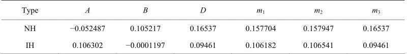
[image:3.595.98.498.596.650.2]U in three different forms e.g. BM, HM as well as TBM and the Table 1. Values of A, B, D, m1, m2, m3.
Type A B D m1 m2 m3
NH −0.052487 0.105217 0.16537 0.157704 0.157947 0.16537
[image:3.595.105.494.679.733.2]IH 0.106302 −0.0001197 0.09461 0.106182 0.106541 0.09461
Table 2. Mass square differences and mixing angles.
2 5 2 21 10 eV
m
2 3 2
31 10 eV
m
Type 2
12
sin 2
23
sin sin13
NH 7.67 2.39 0.37 0.5 0
elements of matrix l are calculated considering it is a Cabibbo-Kobayashi-Maskawa like mixing i.e. [13]:
U
2 3
13
sin l ,
a b
12 23
sinl , sinl , (18)
where varies between 0.104 to 0.247 and a, b varies between 0.2 to 5. From Equation (18) calculated l are used to construct the elements of matrix Ul.
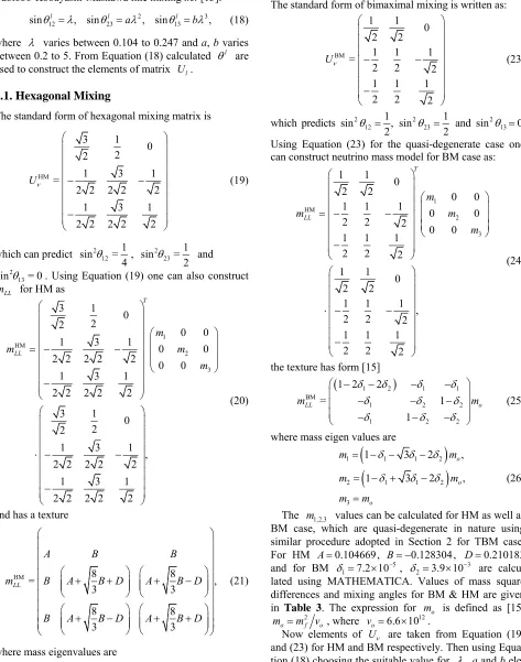
3.1. Hexagonal Mixing
The standard form of hexagonal mixing matrix is
HM
2
= 2 2
2 2
U
3 1 0
2
1 3 1
2 2 2
1 3 1
2 2 2
(19)
which can predict 2 12
1 sin =
4
, 2
23 1 sin = 2 2
sin = 0
and 13 . Using Equation (19) one can also construct
LL
m for HM as
1 2 3 0 0 0 0 0 0 m m m HM 3 1 0 2 2
1 3 1
2 2 2 2 2
1 3 1
2 2 2 2 2
3 1 0
2 2
1 3 1
, 2 2 2 2 2
1 3 1
2 2 2 2 2 T LL m (20)
and has a texture
HM = 8
LL
A B
m B A B D
B A B D A
8 , 3 3 8 8 3 3 B
A B D
B D (21)
where mass eigenvalues are
1 2
2
= , =
3
m A B m A
3.2. Bimaximal Mixing
The standard form of bimaximal mixing is written as:
BM
1 1 0
2 2
1 1 1
=
2 2 2
1 1 1
2 2 2
U (23) 3
6 ,B m = .D (22)
which predicts 2 12
1 sin
2
, 2
23
1 sin
2
2
13 and sin 0. Using Equation (23) for the quasi-degenerate case one can construct neutrino mass model for BM case as:
1 HM
2
3
1 1 0
2 2 0 0
1 1 1 0 0
2 2 2 0 0
1 1 1
2 2 2
1 1 0 2 2
1 1 1
,
2 2 2
1 1 1
2 2 2
T LL m m m m (24)
the texture has form [15]
1 2
1 1BM
1 2 2
1 2 2
1 2 2
= 1 1 LL o m m (25)
where mass eigen values are
1 1 1 2
2 1 1 2
3
1 3 2 ,
1 3 2 ,
o o o m m m m m m m 0.104669 (26)
The 1,2,3 values can be calculated for HM as well as BM case, which are quasi-degenerate in nature using similar procedure adopted in Section 2 for TBM case. For HM A , B 0.128304, D0.210183
and for BM 17.2 10 5 3.9 10 3
m
, 2 are calcu-lated using MATHEMATICA. Values of mass square differences and mixing angles for BM & HM are given in Table 3. The expression for o is defined as [15]
2
m m v 6.6 1012 o
v
U
o f o
Now elements of
, where .
are taken from Equation (19) and (23) for HM and BM respectively. Then using Equa-tion (18) choosing the suitable value for , a and b ele- ments of l have been calculated. Finally deviated
atrix U is constructed using the following equatio
U
n: m
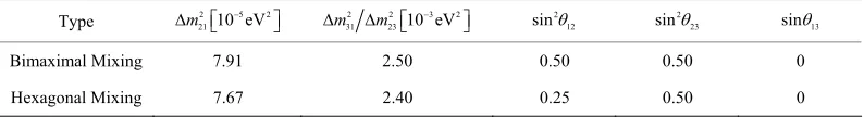
[image:4.595.62.535.107.708.2] [image:4.595.302.540.253.567.2]Table 3. Values of θ12, θ23, θ13 and mass scales.
Type 2 5 2 21 10 eV m
2 2 2
31 23
m m
10 eV3
sin212
2 23
sin sin13
Bimaximal Mixing 7.91 2.50 0.50 0.50 0
[image:5.595.100.497.103.157.2]Hexagonal Mixing 7.67 2.40 0.25 0.50 0
Table 4. Values of θ12, θ23 and θ13.
Mixing type a b 2
12
sin 2 23
sin sin13
Bimaximal Mixing 0.25 0.25 0.18 0.26 0.44 0.047
Hexagonal Mixing 0.3 0.3 0.16 0.31 0.42 0.061
Tri-Bimaximal Mixing 0.3 0.3 0.2 0.29 0.49 0.064
†
13 12 13 12 13 13 12 13 12
PMNS 23 12 12 13 23 12 23 12 13 23 13 23 23 12 12 13 23 12 23 12 13
12 23 12 13 23 12 23 23 13 12 13 23
l l l l l
l l l l l l l l l l l l
l l l l l l l l l l l l
c c c s s c c c s
U U c s c s s c c s s s c s c s c s s c c s s
s s c s c c s c s s c c
s s12 23 c s c12 13 23 c s12 23 c s23 13
13 s
23 13 23
12 13 23
.
s c s
s c c
(27)
This new mixing pattern for suitable value of , and is the new mixing pattern deviated from BM and HM and meet with the recent oscillation data. Values of mixing angles for the pattern along with the suitable parameters are listed in the Table 4 in case of HM, BM as well as TBM.
a b
4. Conclusion
Tribimaximal mixing provides a very close description of neutrino mixing angles. However the present hint of nonzero 13 coming from analysis of global neutrino
oscillation data may indicate that it is broken. Here in this work, we try to use the charge lepton correction in PMNS matrix to get which can predicts recent neutrino oscillation parameters. Different neutrino mixings e.g. TBM, BM, HM as well as tetragonal mixing are well established and can explain the different pattern of neu-trino in context of their mass. Analysis on these mixing are very mass important to give comments on two im-portant aspects e.g. neutrino mass hierarchy and non-zero
13
. In this work we have tried to show quasi-degenerate (NH, IH) property of neutrino by parameterized standard form of neutrino mass matrix using 21, 31 and
i
i considering neutrino is tribimaximaly mix. Then the deviated mixing pattern from TBM, BM and HM have been constructed using charged lepton corrections. From this analysis it can be conclude that neutrino can mix tribimaximaly, hexagonally, and bimaximaly which can predicts the neutrino oscillation parameters accu-rately in
2
m
m2
m
3 level with a small correction in charged lepton part. There is a good scope for extension of this work with CP violating phases. By using 21, 31 and it is also possible to get non-zero
2
m
m2 i
im
13 andsolar and atmospheric mixing angle directly in the range of experimental values.
5. Acknowledgements
Author would like to thank Werner Rodejohann of Max- Planck Institute, Germany for useful discussion during this work. MKD is also supported by start-up grant of Tezpur University, Tezpur.
REFERENCES
[1] K. Nakamura, et al., “Review of Particle Physics,” Jour-nal of Physics G: Nuclear and Particle Physics,Vol. 37, No. 7A, 2010, Article ID: 075021.
doi:10.1088/0954-3899/37/7A/075021
[2] P. F. Harrison, D. H. Perkins and W. G. Scott, “Tri-Bi- maximal Mixing and the Neutrino Oscillation Data,” Physics Letters B,Vol. 530, No. 1, 2002, pp. 167-173. [3] Z. Z. Xing, “A Full Determination of the Neutrino Mass
Spectrum from Two-Zero Textures of the Neutrino Mass Matrix,” Physics Letters B, Vol. 533, No. 1-2, 2002, pp. 85-90. doi:10.1016/S0370-2693(02)02062-2
[4] X. G. He and A. Zee, “Some Simple Mixing and Mass Matrices for Neutrinos,” Physics Letters B,Vol. 560, No. 1-2, 2003, pp. 87-90. doi:10.1016/S0370-2693(03)00390-3
[5] G. L. Fogli, et al., “Hints of θ13 > 0 from Global Neutrino
Data Analysis,” Physics Letters B,Vol. 101, No. 14, 2008, Article ID: 141801.
doi:10.1103/PhysRevLett.101.141801
[6] M. C. Gonzalez-Garcia, M. Maltoni and J. Salvodo, “Updated Global Fit to Three Neutrino Mixing: Status of the Hints of θ13 > 0,” Journal of High Energy Physics, No.
4, 2010, pp. 56-76.
Are on θ13: Addendum to ‘Global Neutrino Data and Re-
cent Reactor Fluxes: Status of Three-Flavor Oscillation Parameters’,” New Journal of Physics, Vol. 13, 2011, Ar- ticle ID: 063004. doi:10.1088/1367-2630/13/10/109401
[8] K. Abe, et al., “Indication of Electron Neutrino Appear- ance from an Accelerator-Produced Off-Axis Muon Neu- trino Beam,” Physical Review Letters, Vol. 107, 2011, Article ID: 041801.
[9] L. Whitehead, et al., “Recent Results from MINOS, Joint Experimental-Theoretical Seminar,” Joint Experimental- Theoretical Seminar, Fermilab, 24 June 2011.
[10] C. H. Albright, A. Dueck and W. Rodejohann, “Possible Alternatives to Tri-Bimaximal Mixing,” The European Physical Journal C, Vol. 70, No. 4, 2010, pp. 1099-1110.
doi:10.1140/epjc/s10052-010-1492-2
[11] Z. Xing, “Tetramaximal Neutrino Mixing and Its Implica- tions on Neutrino Oscillations and Collider Signatures,” Physical Review D, Vol. 78, No. 1, 2008, Article ID: 011301. doi:10.1103/PhysRevD.78.011301
[12] W. Grimus and L. Lavoura, “A Model for Trimaximal Lepton Mixing,” Journal of High Energy Physics, No. 9, 2008, p. 106. doi:10.1088/1126-6708/2008/09/106
[13] S. Goswami, S. T. Petcov, S. Ray and W. Rodejohann, “Large |Ue3| and Tribimaximal Mixing,” Physical Review D, Vol. 80, No. 5, 2009, Article ID: 053013.
doi:10.1103/PhysRevD.80.053013
[14] M. K. Das, M. Patgiri and N. N. Singh, “Numerical Con- sistency Check between Two Approaches to Radiative Corrections for Neutrino Masses and Mixings,” Pra-mana—Journal of Physics, Vol. 65, No. 6, 2006, pp. 995-1013.
[15] N. N. Singh, M. Patgiri and M. K. Das, “Discriminating Neutrino Mass Models Using Type-II See-Saw Formula,” Pramana—Journal of Physics, Vol. 66, No. 2, 2006, pp. 361-375.
[16] G. Altarelli and F. Feruglio, “Discrete Flavor Symmetries and Models of Neutrino Mixing,” Reviews of Modern Physics, Vol. 82, 2010, pp. 2701-2729.
[17] S. Boudjemaa and S. F. King, “Deviations from Tribi- maximal Mixing: Charged Lepton Corrections and Re- normalization Group Running,” Physical Review D, Vol. 79, No. 3, 2009, Article ID: 033001.
doi:10.1103/PhysRevD.79.033001