The application of regression trees to detecting multiple structural breaks in the mean of a time series

THE .APPLICATION OF REGRESSION TREES TO DETECTING MULTIPLE STRUCTURAL BREAKS IN TIIE

MEAN OF A TIME SERIES

Carmela CAPPELLI, William S. REA and Marco REALE 1

Department of Mathematics and Statistics University of Canterbury

Private Bag 4800 Christchurch, New Zealand

Report Number:

The Application of Regression Trees to

Detecting Multiple Structural Breaks in the

Mean of a Time Series

Carmela CAPPELLI, William

S. REA, and Marco REALE

A non parametric approach is proposed for dating structural breaks whose

number and dates of occurrence are a priori unknown. In particular, the case of

level shifts is considered. For the purpose of locating the breakdates the method

exploits, in the framework of least square regression trees, the contiguity property

introduced by Fisher for grouping a single real variable. The proposed approach

is applied to study the changes in growth rates in Campito Mountain bristlecone

pines, a standard example of a long memory time series.

Key Words: Fisher's algorithm; Least square regression trees; CUSUM; Bai and

Perron procedure.

1 INTRODUCTION

The detection of structural breaks is an important problem in time series

analysis that has attracted the attention of both statisticians and

econome-tricians for more than forty years (for a review see Hansen 2001). In this

1_{Carmela Cappelli is a Researcher, Department of Statistical Sciences, Universita}

di Napoli Federico II, Via L. Rodino n.22, Naples, I-80138. William Rea is a PhD student, Mathematics and Statistics Department, University of Canterbury, Private Bag 4800, Christchurch. Marco Reale is a Senior Lecturer, Mathematics and Statis-tics Department, University of Canterbury, Private Bag 4800, Christchurch. (E-mail:

paper we focus on the problem of detecting multiple breaks occurring at

unknown dates. To this aim, recently, Bai and Perron (1998, 2003) have

pro-posed an estimation procedure that makes use of a dynamic programming

approach that can be traced back to Fisher's method of exact optimization

(Fisher, 1958) for grouping a single real variable into mutually exclusive

and exhaustive subsets having maximum homogeneity, i.e. minimizing the

within-group sum of squares.

Regression trees (RT) are a non-parametric method for fitting piece-wise

constant functions to a data set. The boundaries between the constant

func-tions are steps. These are often regarded as a drawback or weakness if the

variable being modeled is continuous. However, change point analysis is

un-dertaken when it is believed that the underlying data generating process is

discontinuous, or at least changes rapidly between two distinct states, at

the change or break point. In this context it seems natural to interpret the

discontinuities in the RT as the break points in the process. There is a

sub-stantial body of literature dealing with change point detection and location

in time series. However, apart from the papers of Cooper (1998) and

Cap-pelli, Penny, Rea and Reale (2007) the application of RT to this problem

appears to be an overlooked tool.

In this paper we describe the use of RT in the location of structural

(3) presents the results of a simulation study on using RT to find

struc-tural breaks in the mean. Section (

4)

the changes in the tree-ring index of Campito Mountain, California. Brief

concluding remarks follow in Section

(5).

2 REGRESSION TREES

Hyafil and Rivest (1976) showed that the problem of obtaining an optimal

binary decision tree is NP-complete. Thus, with the exception, of small data

sets, it is computationally impractical to search for an optimal tree. Despite

their sub-optimal results, RT have found wide application owing to their

computational efficiency. This allows them to handle large data sets with

relative ease. Probably the best known regression tree methoclology is the

Classification and Regression Tree ( CART) of Breiman, Friedman, Olshen

and Stone (1984) to which the reader is referred for a detailed description of

RT.

The recently proposed procedure of Bai and Perron (1998, 2003) (BP) is

based on Fisher's (1958) method of exact optimization. While the BP

pro-duces an optimal partition of a time series, it is a computationally expensive

procedure.

volatilities, tree-ring indices, mud-varve sequences, and ice core data are very

long. Sometimes the geophysical series exceed 10,000 data points with annual

resolution. The long compute times and large memory requirements of the

BP makes its use impractical on these types of series. We show that RT

provide a practical alternative for locating structural breaks in the mean of

long time series data. In the context of RT time assumes the role of the

predictor variable when, in fact, it is merely a counter. A common source of

poor predictive performance in RT is that the distribution of the response

variable is not orthogonal or parallel to the predictor variables (see Fig 8.12

of Hastie, Tibshirani and Friedman 2001, for an example). This problem

does not arise in univariate time series. This gives us reason to suspect they

will perform well in the location of structural breaks.

There are several questions to be addressed in applying RT to time series.

These

are:-1. As RT fit piece wise constant functions to data do RT discover or

impose breaks on time series?

2. What is the effect of serial correlations on RT performance in detecting

structural breaks?

3. Given that observations in time series are, in general, non-interchangeable

Consider the time series model:

Yt

=

+

=

=

+

where G is the number of regimes ( and G -1 the number of breakdates), Yt is

the observed response variable and f.t is the error term at time

t

common convention that To= 0 and Ta= T where Tis th~ series length).

This is a pure structural breaks model because all the model coefficients are

subject to change and it has been employed by Bai and Perron (2003) to

detect abrupt structural changes in the mean occurring at unknown dates.

The problem is to estimate the set of breakdates (T1 , ... , T9, .•. , Ta-i) that

define a partition of the series

P(G)

=

+

+

... ~,_,;.,;:;,

·~

into homogeneous intervals such that µ₉

i=

is based on the least squares principle: for each G-partition, the

correspond-ing least square estimates of the µ₉ 's are obtained by minimizing the

within-group sum of squares

G T9

WSSylP(G) =

I: I:

µg)2.

(2)

g=l t=T₉-1+l

The estimated breakdates

(T'

T

Ta-

par-titian P*(G) such that P*(G) = argminP(G) WSSvlP(G)· In this approach,

all possible partitions by using the dynamic programming approach proposed

by Fisher,s (1958) to find the least squares partition of T contiguous objects into G groups. His efficient algorithm exploits the additivity of the sum

of squares criterion using a dynamic programming approach (Bellmann and

Dreyfus 1962) that when applied to ordered data points finds the global

min-imum. Despite the computational saving, the method cannot deal with high

values of T and G and the same remark holds for the BP,s procedure, even

with todais computing power.

In the case of time series data Hartigan (1975) provides an excellent

justification in favor of the (faster) binary division algorithm: suppose that

the observed time series consists of G segments within each of which the

values are constant, i.e. model (1) becomes a piecewise constant model with

f.t = 0. The series can be partitioned into G segments where for each segment

the within-group sum of squares is zero. This partitioning can be identified

by a sequential splitting algorithm such as the one in RT.

The binary splitting used by RT does not necessarily provide the optimal

partition, however if the correct number of partitions is identified, because

the observations are ordered by time, misplacements can occur only on the

boundaries. As discussed in Hansen (2001), although structural breaks are

treated as immediate, it is more reasonable to think that they take a period

concern.

Despite the potential suboptimal solutions, RT has the advantage over

global search algorithms as used in BP method in being computationally

fast. The global search algorithm requires O(n2

) steps, whereas RT, at any

tree node requires O(n(h)) steps to identify the best split, where n(h) is the

number of values in node h.

Another distinction between RT and the global search algorithm is in the

selection of the final partition and the consequent set of break dates.

In-deed, partitioning methods such as Fisher's (and BP's) have the drawback

of producing a single partition for a prespecified value of G and, in general,

it is advisable to produce and compare more partitions by varying G. In the

case of RT this is not a concern because the method produces a hierarchical

tree structure associated with the breaks. The selection of the final set of

breakdates can be handled within the framework of tree methods by pruning.

Pruning is the process of retrospectively discarding branches whose

contribu-tion to the reduccontribu-tion of the error is negligible (for details see Breiman et al.

1984, Chap. 3). In this way a nested sequence of partitions and candidate

breakdates is created. In order to select the optimal sequence

correspond-ing to the actual number of break dates and distinct subperiods present in

the data, cross validation (CV), the sequential testing procedure of BP and

selection criteria in regression trees see Su, Wang and Fan 2003). Moreover,

the inspection of the tree structure allows an insight into the partitioning

process. Breakdates can be ordered based on their position in the tree and

the reduction of the error function achieved. For this reason manual pruning

based on subjective choices of the analyst can be preferre1 to an automatic

procedure, see Zhang and Singer (1998, Chap. 4).

Finally, note that if estimation is not the sole concern and one wants to

test for structural breaks or model the observations in the segments, it can be

appropriate to consider restrictions on the possible values of the breakpoints

as suggested by BP. Indeed, extra conditions on the reduction in deviance

and/or on the length of the subperiods are easily handled within the tree

growing recursive partitioning approach of RT.

3 SIMULATION EXPERIMENTS

In this section we present the results of simulation experiments using RT to

detect structural breaks. For comparison purposes we used the estimation

procedure proposed by BP based on the Fisher's method of exact

optimiza-tion.

For the RT method we used tree growing and pruning procedures as

BP method we used the contributed package strucchange (Zeileis, Leisch,

Hornik and Kleiber 2002) in R.

3.1

A set of simulations were run with series of uncorrelated observations drawn

from standard Normal, geometric and gamma distributed populations with

a single break point at the midpoint of the series giving two equal lengthed

regimes. In most simulations there where 16 regime sizes, 52 _{to 20}2

obser-vations in length. Thus in the graphs of the results the axis labeled Regime

Number is non-linear in scale. The break sizes ranged from 0.05 to 2

stan-dard deviations in steps of 0.05 stanstan-dard deviations. 1,000 replications of

each combination of regime length and break size were run. For the

com-parable results from the BP the break sizes ranged from 0.1 to 2 standard

deviations in steps of 0.1 standard deviations. The longest series were

com-posed of 256 data points per regime (regime 16). 100 replications were run

of each parameter combination. The results for the standard normal

simu-lations are presented here, the remainder are available on request from the

authors.

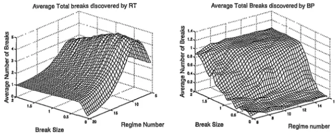
Figure (1) presents the results for the RT and BP for a single break at

Average Total breaks discovered by RT Average Total Breaks discovered by BP

,,,.,

J:;

rr ;

r1: ,

...

··· ···

0 1 ...

16

Break Size

Break Size Regime Number Regime number

Figure 1: Left panel: Average total number of breaks found by RT. Right panel: Average total number of breaks found by BP. Simulated series of un-correlated observations with Gaussian noise and a single break. Pruning based on cost complexity using deviance. Break size is measured in terms of standard deviations. Regime number refers to the length of the series, regime 5 is length 52 and the series is 2

x

series is 2

x

reversed in the BP results compared to the RT results. When the series are

short the RT is very prone to over-fitting but that this tendency gradually

disappears by a series length of approximately 700 data points (regime 18 or

19). RT had a tendency to over-fit for smaller breaks and for shorter regimes.

BP tended to under-fit for smaller breaks and for shorter regimes.

We tested the RT ability to find the location of the break when the break

Total Breaks discovered by RT

en ~ 1.4 ,•'

(I)

[O 1.2

'51

] 0,8 ,,,

~ 0.6

Z 0.4 (I)

g' 0.2

Q) 0 ~200

.... ....

Break Location

··r· ·· ...

,.,···:·, ':···· ...

.... ·· .. : ..

0 0

..

::)"··

···· ... ! .. ·::.:.:.:.l:::::.

Break Size

2

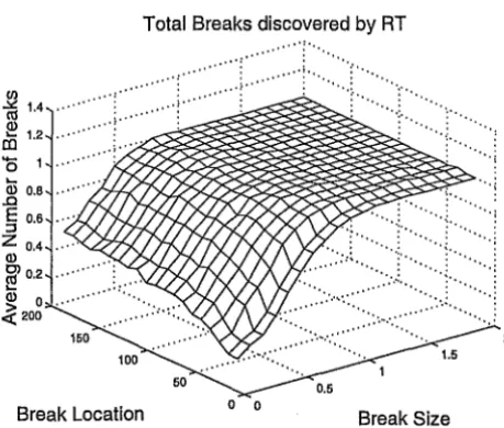
Figure 2: Average total number of breaks found by RT. Simulated series of

400 uncorrelated observations, Gaussian noise and a single break at different

locations. Pruning with Bayesian Information Criterion.

examined series with 100, 400, and 1600 observations. The BP was not run

for comparison. We present the results for the 400 data point series, the

remainder are available on request from the authors.

The results are presented in Figure (2). The dominant factor in locating a

break is its size rather than its location. Unsurprisingly, it was more difficult

3.2

To investigate the performance of RT for series with multiple breaks we

simulated series with 4 breaks:

(3)

where

µr;

=

=

Et

=

In all simulations µr;

=

=

=

started at 2 standard deviations and was decremented to 0.05 in steps of 0.05.

When the BP was used to detect breaks in the series, because the amount of

computation required, the value of µr2 was sometimes decremented to 0.1 in

steps of 0.1.

The resultant series were square waves with an amplitude of break size

with Gaussian ( or other) noise of constant variance imposed on them. We

present the results for the Gaussian noise series. The remainder are available

on request from the authors.

We also examined three tree-pruning methods. The deviance-based cost

complexity, the default method in the R package, the Bayesian Information

infor-mation criteria available we selected the BIO on the basis of Su et al. (2004) and because it is more robust to non-Gaussian error structures than the AIC

(Akaike 1970).

Total breaks discovered by BP

16

Break Size

Regime Number Break Size _{Regime number}

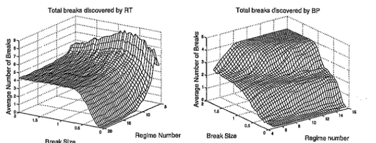
Figure 3: Left panel: Total number of breaks found by RT in the noisy square wave simulations. Deviance based cost-complexity pruning. Right panel: To-tal number of breaks found by BP. The series have four breaks and Gaussian noise.

It is well-known that tree-based procedures over-fit small datasets (Cooper

1998). Thi~ can be seen in the left panel of Figure (3). However, as the series

lengthens the problem of overfitting reduces and is not evident by regime 15

(length of about 1000 data points). This is where the compute times of the

BP begin to become excessive. The BP method underfit for small breaks

particularly for for short series.

Total breaks discovered by RT Total breaks discovered by RT

0.6 20

Break Size Regime Number Break Size Regime number

Figure 4: The average total number of breaks found by RT when using BIG

pruning (left panel) and leave-one-out cross-validation (right panel). The

series have four breaks and Gaussian noise.

aggressive pruning criteria than the usual R-default cost-complexity pruning

introduced by Breiman et al. (1984). The results of BIC and

leave-one-out cross-validation are presented in the left and right panels of Figure ( 4)

respectively.

In time series data observations are usually not interchangeable. Thus the

common 10-fold cross-validation cannot be used. The alternative we

consid-ered was leave-one-out cross-validation. This minimizes the disturbance to

any correlation structure in the data but it is much more computationally

expensive than the BIC, requiring N trees to be constructed where N is the

number of data points. The leave-one-out cross-validation pruning reduced

for its robustness to non-Normality, but note that for series with more than

approximately 600 data points the BIC becomes indistinguishable from the

default cost-complexity pruning.

3.3

To investigate the ability of RT and BP to detect structural breaks in

corre-lated data we analyzed series with AR(l), AR(2), AR(5), and MA(l)

correla-tions. The results for the AR(l) series are presented here and the remainder

are available on request from the authors.

Average Total breaks discovered by RT

AR(1) Parameter Break Size

i ~

~

:0 •

0 "

Cl)

0 •

E

:,

z •

~ Iii •

~

Number of Breaks Discovered by BP

..

..

AR(1) Parameter

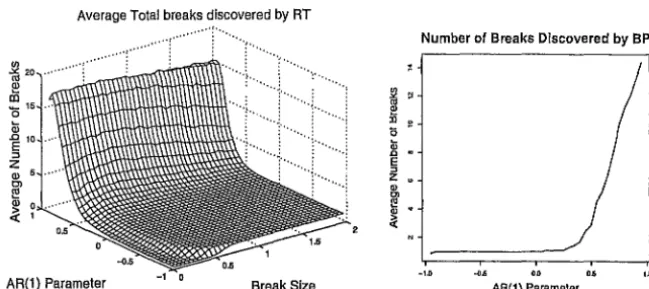
Figure 5: Left panel: Average total number of candidate breaks found by RTs in series with AR(i) correlations and a single break. Default pruning. Right panel: Comparable results from the BP for a break size of two.

The left panel of Figure (5) show the results for the RT. The right panel

the results of the BP for a break size of two standard deviations. All series

were 1024 observations long. It should be noted that the series standard

deviation changes with the magnitude of the AR parameter. The break size

was measured in terms of the input noise series.

Both RT and the BP are robust to negative values of the AR parameter

and to small positive values (less than 0.25). However, neither break

detec-tion method is robust to larger positive values, each finds increasing numbers

of spurious breaks as the AR parameter approaches unity.

We found that the RT had similar robustness to MA correlations except

that they induced far fewer spurious breaks when the MA parameter was

higher than 0.25. In the worst case an average of less than one spurious

break per series was reported.

3.4

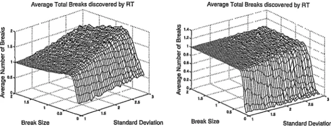
We examined RT robustness to heteroscedasticity by simulating series with

a break at the mid-point and different standard deviations in the two halves.

The first half always had a standard deviation of one. The break size is

stated in standard deviations of the first half. The second half had a standard

deviation ranging from one to 2.95. We examined two lengths of series, 800

and 1800 data points. We did not run BP for comparison due to the excessive

Average Total Breaks discovered by RT

i

~u

···r

Break Size

··r ... , ... ,

... .

Standard Deviation Break Size _{Standard Deviation}

Figure 6: Average total number of breaks found by RT in series with

het-eroscedasticity. Left panel - 800 data point series. Right panel - 1800 data

point series. Deviance-based cost-complexity pruning. The series had one

true break.

The results are presented in Figure (6). RT is more robust to

het-eroscedasticity in the longer series than in the shorter series. This is

consis-tent with the other observations presented in this paper that the problem of

over-fitting declines with increasing series length.

4 APPLICATION: CAMPITO MOUNTAIN TREE

RING INDEX

To illustrate the RT method in comparison to the BP method we applied both

methods to the Campito Mountain bristlecone data. The dataset is available

/Books/HipelMcLeod/lamarche/ campi to .1 and is also available in the

li-brary of the contributed package tseries in R. These data are regarded as a

standard example of a long memory process (see Doukhan, Oppenheim and

Taqqu 2003). Klemes (1974) argued that the appearance of long memory

in geophysical time series was often a statistical artefact caused by a

non-stationary mean. Despite Klemes' arguments and numerical experiments he

could not demonstrate the correctness of his proposal from data analysis.

The physical cause or causes of long memory is still an open question. We

examine the Campito data with RT and BP to see if a non-stationary mean

can be detected.

We ran the BP on the Campito data twice. The first time with the

mini-mum segment size set to 0.05 times the length of the series or approximately

270 data points. The second time with the minimum segment size set to 0.01

or approximately 54 data points. The second run took almost 243 hours of

CPU time on a SunBlade 1000 with 750Mhz UltraSPARC-III processor and

2Gb of memory. By comparison the RT took 0.16 seconds. This supports

our contention that regression trees are a practical, if sub-optimal, tool for

analyzing long time series.

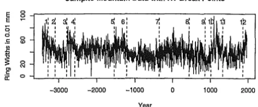
Figure (7) presents the Campito data with the break points marked for

both the regression tree and the BP with the minimum segment size set to

Campito Mountain Data with RT Break Points

E 0 0

E ~

~

0

d

0

.5 co

U)

.c

i5

~ 0

C) (\J

c

ii: 0

-3000 -2000 -1000 0 1000 2000

Year

Campito Mountain Data with BP Break Points

E 0 0

E ~

ci

0 0

.5 co

U)

=

'O

~ _1il

C)

.5

0

[(

-3000 -2000 -1000 0 1000 2000

Year

Figure 7: Regression (RT) and Bai and Perron (BP) break points marked on

the Campito data.

the break points are essentially identical. With a minimum segment size of

0.01 the BP reported 40 break points. We regard 40 breaks to be an excessive

number and do not report them here. They are available on request from the

authors. We attribute the difference in the reported numbers of break points

between the RT and the BP to be due to the penalty terms applied in pruning

CUSUM with RT Breakpoints - Campito Mountain Data

1: 2:

s:

II) I

Q) _ex, I

~

(l) I

I

::;; _'St

::,

en N

::, (.)

0

-3000 -2000 -1000 0 1000 2000

Year

CUSUM with BP Breakpoints - Campito Mountain Data

1' I 2:

s:

s:

II)

Q)

<D ::,

iii

> (l)

::;; _'St

::,

en N

::, (.)

0

-3000 -2000 -1000 0 1000 2000

Year

Figure 8: Regression tree (RT) and Bai and Perron (BP) break points marked

on CUSUM graphs for the Campito data.

trees. It is not clear how to select the optimal number of breaks in the BP.

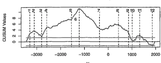
Figure (8) presents both the tree and BP break points on a cumulative

summation (CUSUM) (Brown, Durbin and Evans 1974) graph. The CUSUM

graph in interpreted subjectively by examining the slope of the plot with

regard to the five percent significance lines plotted parallel to the horizonal

an above average growth rate. Conversely, when the slope is negative the

tree is experiencing below average growth. In these plots there are several

places where the RT breaks appear more physically reasonable than the BP

breaks.

The first is the regime between breaks three and four in RT, which most

closely relate to breaks two and three in the BP. The RT places the break at

the end of a period of above average growth while BP includes a short period

of below average growth. Similarly RT breaks nine through 12 seperate out

the above and below average growth periods. In the corresponding period BP

breaks 11, 12, and 13 generate regimes which mix above and below average

growth rates.

One the other hand, for break point six, the RT places this at the highest

point on the CUSUM plot whereas the BP displaces this slightly to the left.

Examining the break points in Figure (7) the BP break point appears the

more reasonable.

5 CONCLUDING REMARKS

We have proposed a new application of RT by using them as a data driven

nonparametric procedure for detecting multiple structural breaks in the mean

to our three original questions. They are,

1. RT do impose spurious breaks when the series is short but this tendency

disappears as the series becomes longer. This was seen in both single

and multiple break simulations.

2. RT are robust to negative serial correlation and a small amount of

positive correlation, but in this regard they are no worse than the BP.

3. Leave-one-out cross-validation can be used for tree selection but is

com-putationally expensive.

The main advantages of the proposed approach are:

1. simplicity -it can be easily implemented or run with packages contain-ing routines to grow and prune least squares regression trees;

2. feasibility - it can be used to find the least squares partition of an ordered sequence and is particularly suited to long series which are

currently not practical to analyse with the BP;

3. visualization - it results in a nested hierarchy represented by a tree diagram that displays the whole partitioning process and allows the

scientist to interact with the tree and make use of a priori knowledge. Although RT do not necessarily find the global minimum, their results

series are long. In the example data set the breakdates for both the RT and

BP coincide at a number of points. Also, in our example data set some of

the RT break points are more physically reasonable than the optimal break

points of the BP.

The application to the Campito Mountain data shows that Klemes'

con-tention that the Hurst effect is caused by a non-stationary mean is supported

by both the RT and BP. However, the RT is computationally orders of

mag-nitude faster than the BP for this series.

As with any statistical test or modelling procedure, regression trees must

be used with care and discernment. For an experienced time series analyst

who must deal with long series, RT provide a complementary procedure to

the BP when detecting and locating structural breaks in the mean.

Acknowledgements. Carmela Cappelli acknowledges financial support

from Dipartimento di Scienze Statistiche.

References

Akaike, H. (1970), "Information Theory and an Extension of the Maximum

Likelihood Principle," in 2nd International Symposium on Information

Theory, eds. B.N. Petrov and F. Csaki, Budapest: Akademia Kadio,

Bai, J., and Perron, P. (1998), "Estimating and Testing Linear Models with

Multiple Structural Changes," Econometrica, 66, 47-78.

Bai, J., and Perron, P. (2003), "Computation and analysis of multiple

struc-tural change models," Journal of Applied Econometrics, 18, 1-22.

Bellmann, R. E., and Dreyfus, S. E. (1962), Applied Dynamic Programming,

Princeton: Princeton University Press.

Breiman, L., Friedman, J. H., Olshen, R. A., and Stone, C. J. (1984),

Clas-sification and Regression Trees, Monterey (CA): Wadsworth & Brooks.

Brown, R. L., Durbin, J. and Evans, J. M. (1974), "Techniques for Testing

the Constancy of Regression Relationships over time," Journal of the

Royal Statistical Society B, 37, 149 - 163.

Cappelli, C., Penny, R. N., Rea, W. S., and Reale, M. (in press),

"Detect-ing Multiple Mean Breaks at Unknown Points with Regression Trees,"

Mathematics and Computers in Simulation.

Cooper, S.J. (1998), "Multiple Regimes in U.S. Output Fluctuations,"

Jour-nal of Business and Economic Statistics, 16, 92-100.

Doukhan, P., Oppenheim, G., and Taqqu, M. (2003), Theory and

Fisher, W.D. (1958), "On Grouping for Maximum Homogeneity," Journal

of the American Statistical Association, 53, 789-798.

Hansen, B. E. (2001), "The New Econometrics of Structural Change:

Dat-ing Breaks in the U.S. Labor Productivity," Journal of Economic

Per-spectives, 15, 117-128.

Hartigan, J. A. (1975), Clustering Algorithms, New York: John Wiley &

Sons.

Hastie, T., Tibshirani, R., and Friedman, J. (2001), The Elements of

Sta-tistical Learning, New York: Springer Verlag.

Hyafil, L., and Rivest, R. (1976), "Constructing Optimal Binary Decision

Trees is N-P Complete," Information Processing Letters, 5, 15-17.

Klemes, V. (1974), "The Hurst Phenomenon: A Puzzle?" Water Resources

Research, 10, 675-688.

Morgan, J. N., and Sonquist, J. A. (1963), "Problems in the Analysis of

Sur-vey Data and a Proposal," Journal of American Statistical Association,

58, 415-434.

Schwarz, G. (1978), "Estimating the Dimension of a Model," Annals of

Su, X. G., Wang, M., and Fan, J. J. (2004), "Maximum Likelihood

Regres-sion Trees," Journal of Computational and Graphical Statistics, 13,

586-598.

Zeileis, A., Leisch, K., Hornik, K., and Kleiber, C. (2002), "Strucchange:

an R Package for Testing for Structural Breaks in Linear Regression

Models," Journal ofSta#stical Software, 7, 1-38. ·

Zhang, H., and Singer, B. (1998), Recursive Partitioning in the Health