Metaheuristic Robust Optimization of Project Portfolios using an Interval Based Model of Imprecisions

Received Jan 29, 2016 / Accepted Aug 21, 2016

Editorial Académica Dragón Azteca (EDITADA.ORG)

Metaheuristic Robust Optimization of Project Portfolios using an Interval-Based Model of

Imprecisions

Fausto Balderas11_{, Eduardo Fernandez} 2_{, Claudia Gómez} 3_{, Laura Cruz-Reyes}3

_{, Nelson Rangel-Valdez}

4

1 _{National Mexican Institute of Technology/Tijuana Institute of Technology, México,} 2_{Autonomous University of Sinaloa,} México, 3_{National Mexican Institute of Technology/Madero Institute of Technology, Mexico,} 4_{CONACYT Research Fellow,}

National Mexican Institute of Technology/Madero Institute of Technology, México.

[email protected], [email protected], [email protected], [email protected] [email protected]

.

Abstract. Organizations often approach portfolio optimization problems. In many practical cases, the decision-maker faces uncertainty relating to future uncertain states of nature that cause variability in project benefits, in resources to be consumed by the project and resources available to support the portfolio, this often carries uncertainty, due to cognitive limitation of human beings, a great quantity of deal of the information of interest. We used an interval approach for describing and representing uncertainty associated with problems of real-life decision-making. The aim of this work is to provide an approach of handling the uncertainty found in project portfolio selection using grey numbers, which are a way of interval numbers. A fundamental step of our proposal was to generalize NSGA-II for the treatment of multi-objective grey optimization problems. Our proposal provides a better quality of solution concerning the treatment of uncertainty.

Keywords: project portfolio selection,uncertainty, interval approach, multi-criteria optimization.

1. Introduction.

Resource allocation problems are ubiquitous in enterprises and governmental organizations ([22]). Projects require resources and the organization faces the problem how to distribute them in order to meet organizational objectives. The problem consists of selecting a subset of projects that together contribute, in the best possible way, to the accomplishment of objectives of the organization that distributes the resources. This strategic decision problem is known as project portfolio selection. And it can be raised in his general form as follows:

Let us suppose that there is a finite set A of N projects, each described by estimates of its impacts and resource consumption. A portfolio is a subset of A that can be represented by a binary component vector X  x x₁, ₂,...,x_n , where the value “1” of the component

x

_i indicates that the i-th project is the one that will be financed.

Portfolio consequences are usually described by multiple attributes related to organizational goals and objectives. A vector of impacts z x

 

 z x₁

   

,z₂ x ,...,z_p

 

x is associated with consequences of portfolio X considering P criteria. In a simpler case z x

 

is obtained through the sum of benefits of the selected projects. Without loss of generality, we can assume that higher values of criteria are more preferable than lower values. The best portfolio is obtained by solving Problem 1:

   

 





1 , 2 ,..., p F

Maximize z x z x z x

xR

, (1)

where RF is the space of feasible portfolios, usually determined by the available budget and by other constraints that the Decision Maker (DM) wants to impose (e.g.: budget limits on types, geographic areas, or social roles of projects). This problem has been approached by many scientific paper (e.g. 5, 6, 23, 35, 43).

102

Portfolio decision analysis (PDA) can be defined as a body of theories, methods and practices which helps decision makers to select a subset from a very large set of projects through mathematical modeling taking into account relevant constraints, preferences, uncertainty or imprecision ([38]).

The difficulty of PDA-related problems comes from some of the following factors or their combination:

Large size of entry space. It’s a decision-making problem with exponential complexity even when decisions are about allocating or not the resources to each of candidate projects. The complexity increases when decisions about partial support to projects are admitted.

Multidimensional consequences of projects and portfolios. This problem requires a multi-criteria description in terms of usually conflicting attributes. Sometimes, the solution space is bi or three-dimensional. But in more complex problems, the amount of dimensions may easily exceed human cognitive capabilities for evaluating different candidate solutions ([17]).

Qualitative, imprecise or uncertain information. Qualitative information is difficult to handle using optimization methods. The contribution of projects to portfolio measures is often not accurately known, that is, there exists imprecision due to lack of knowledge about future states of nature (probabilistic uncertainty), or due to a simple lack of information (vagueness), which strictly speaking is very difficult to model using probability distributions. Information on the time and resources required to complete the projects as well as total resources available to DM may also be imprecise. Vague approximations and areas of ignorance, which affect modeling and data, limit the scientific approach in Operational Research-Decision Aiding ([37]). In the following we refer those imperfections under the umbrella term of “uncertainty”.

It is assumed that the DM’s system of preferences and values reflects appropriately the aspirations of the organization that distributes resources. Solving a multi-objective version of Problem 1 means to find a solution portfolio that best satisfies DM´s preferences on conflicting criteria. Most of the researches in the literature are dedicated to the mathematical and algorithmic complexities of Problem 1 and to the modeling of the DM’s preferences. However, significant elements of uncertainty that affect the evaluation of impacts and the very definition of feasible region are often involved in this process. Roy in [37] defines a frailty point as a place in the model, or in procedure processing the model, where uncertainty can be found. To meet the concern for robustness properly, careful inventory and consideration of all frailty points the formal representations are required ([37]). In Problem 1 the most remarkable uncertainty is often found in project multi-dimensional impacts, project resource consumptions, and total amount of available resources. Following [37], the term robust is a qualifier that refers to an aptitude to withstand uncertainty, to provide protection against deplorable results that are much worse than expected. This qualifier applies to solutions, conclusions, recommendations and methods. Robustness is a concern that has to be taken into account. However, there are relatively few researches devoted to address robustness in Problem 1.

This contribution is intended to present a new method of handling uncertainty and obtaining more robust solutions in multi-objective optimization portfolio problems by using “grey” numbers that are expressed as intervals of real numbers to reflect the imprecision of a magnitude. Interval analysis is a method originated independently by Sunaga [44] and Moore [32] and developed ever since the 1950s by a score of mathematicians as an approach to putting bounds on rounding errors and measurement errors in mathematical computations. Grey mathematics is a variant of interval analysis with specific properties. Liu et al. in [10] states that interval analysis should be seen righteously as a proper sub-portion of grey mathematics. Section 2 discusses some approaches on how to reflect uncertainty in the problem of project portfolio selection. Section 3 presents the conceptual basis that allows grey numbers to be used in the solution of Problem 1, generalizing several concepts of optimization to grey environment. Section 4 describes methods we propose for portfolio optimization using grey mathematics and an extension of a popular multi-objective evolutionary algorithm to that environment. Section 5 provides details on computational experiments made, which show the elegance of our proposal and its advantages with respect to traditional heuristic approaches to handling uncertainty. Lastly, our conclusions are given in Section 6.

2. A general overview of different approaches to modelling uncertainty in the problem of project portfolio selection.

103

of what will happen in the future; that is to say, from this perspective, it has negative implications for projects, as it obviously limits investments. Uncertainty is also applied in decision-making; indeed, this sort of circumstance has enormous relevance at the time of deciding whether to follow one or another route in a determined project. Let us distinguish two types of uncertainty:

First, uncertainty relating to future uncertain states of nature that cause variability in project benefits, in resources to be consumed by the project and resources available to support the portfolio. Second, the imprecision associated with vagueness, non-stochastic imprecise knowledge. Probability and fuzzy set theories are tools that are generally used to approach these issues.

Probabilistic modeling has been chiefly applied to handle the variability of projects’ impacts. Many papers introduce additional criteria into the problem of optimization (1) trying to minimize a risk measure. Various researches differ regarding the definition of this measure (cf. [3, 14, 23, 32, 34, 40]). To our knowledge, distributions of probability have not been used to model the imprecision in resources required by the projects.

Fuzzy Set Theory has been usually applied for modeling not only the imprecision in impacts, but also the vagueness of resources and flexible information of projects ([46]). By using fuzzy set-based modeling, benefits and imprecisions are added in a fuzzy manner through operators. The way in which these operators model the attitude in the face of DM’s uncertainty and the manner in which he/she counterbalances risks and benefits can be questioned. The results depend on the election of aggregation operator, and in the absence of a regulatory structure of the fuzzy logic, there isn’t one sole way to do it.

For instance, Lin and Hsieh [28] and Wei and Chang [47] used linguistic variables to model imprecise information about criteria. Damghani et al. in [9], Huang in [19] and Kuchta in [24] employed fuzzy numbers to model requirements of resources and imprecise benefits. Bhattacharyya et al. in [4] solved a fuzzy problem of three-objective optimization by maximizing a measure of benefit and minimizing costs and risks.

Liesio et al. proposed Robust Portfolio Modeling (RPM) in [25, 26]. Using a weighted sum function model, this approach identifies solutions for which no other feasible portfolio yields greater value for all possible realization of the uncertain project scores and criterion weights. By requiring greater value for all possible realization of uncertain parameters, RPM is probably a very conservative approach. Inspired on RPM, a more flexible approach that allows adjustments to the level of conservatism has been recently proposed by Fliedner and Liesiö in [18].

Due to complexity and uncertainty present in decision-making, as well as to cognitive limitation of human beings, a great deal of the information of interest, such as project benefits, resources to be consumed by the project and resources available to support the portfolio, are obtained through gross estimates or usually inaccurate data collection. A natural and simple way to express the imprecision inherent to this information is through intervals of uncertainty, without the need to specify whether it is due to variability of states of nature or to vagueness of information.

The grey approach is a novel tool for describing and representing uncertainty associated with problems of real-life decision-making. Grey numbers have been applied in many real-world problems, such as manufacture (e.g. [21, 39]), hydrology (e.g. [1]), decision-making (e.g. [45]), medicine (e.g. [15]), and risk assessment (e.g. [31]). The grey approach was applied by Arasteh and Ahliamadi in [2] to portfolio project selection in combinations with Real Option Theory. To the best of our knowledge, there have been no researches that applied the grey approach to the treatment of uncertainty related to impacts and resources in the frame of Problem 1. The application of grey mathematics allows an easy adjustment of the level of conservatism. Thus, the DM can select a final best compromise in accordance with his/her preferences, beliefs and attitude toward uncertainty. This contribution intends to provide a deep look on this area.

3. Theoretical basis.

3.1.Fundamental concepts of grey arithmetic.

104

the treatment of project portfolio problems. A grey number is an entity that reflects a quantitative property whose exact value is unknown, but the range within which the value lies is known.

A grey number is generally denoted by " " and is represented in terms of a range as   A A A, _where A is the lower limit and A is the upper limit of the grey number ([30]).

A real number a belonging to the interval _A A, _is said to be a realization of the grey numberA.

Shi et al. in [41] define certain sorting relation rules over grey numbers. First, the measure of possibility of   D Eis introduced through Equation 2:













*

*

max 0,L max 0,D E

P D E

L

 

    , (2)

where L



D







DD



is the length of grey number D and L*L



D

  

L E .

The sorting relation between D and E is determined as follows:

(i) If DE andDE, it is said that D is equal toE, denoted as   D E. Then P



  D E



0.5.

(ii) IfED, it is said that Eis greater thanD, denoted as   E D. ThenP



  D E



1.

(iii) IfED, it is said that Eis smaller thanD, denoted as   E D. Then P



  D E



0.

(iv) If D E DE or D  E E D, when P



  D E



0.5, it is said that E is greater than D, denoted as

E D

   When P



  D E



0.5, it is said that E is smaller than D, denoted as   E D.

When P



  D E











0.5



we say that E is



greater thanD, denoted as  E _ D.  is called the support of  D E.Let d and e be two currently undetermined realizations from D and E, respectively;  can be interpreted as a degree of credibility of the statement “once both realizations are determined, e will be greater or equal than d”. This helps the DM to ensure the robustness of  D E, that is: to have a strong belief on E is not less than D

when they are instanced as real numbers.

3.2.Mono-objective grey optimization problems.

We will introduce the following concepts for our work:

Definition 1:We will call greyvector an n-tuple of grey numbers, symbolized by:

1, 2,..., n

x x x x . (3)

Definition 2: A grey function of grey variables is an application of a set of grey vectors

 

X in a set of grey numbers

 

Y , such that each element x of

 

X matches an element yof

 

Y ;

: ,

f x y

    (4)

where the set

 

X is the domain of function (DomF) and the set

 

Y is the image of function (ImF) .

Variables of the domain of function are called decision variables, that are adjustable within a grey optimization problem; they are instantiated as grey numbers and their values are denoted as: x_j for j1, 2,..., .n

Definition 3: Maximum of a grey function: It is a grey number of the image of function such that it is greater than or equal to all grey numbers belonging to the image of grey function:

 

max| max

Im .F

Maximum f x

y y y

y

  

   

  

105

Definition 4: Maximizing a grey function, is the process of finding the grey vector of domain where the function takes a maximum value:

 

Maximizingf x . (6)

Definition 5: We will call greyobjective function a grey function that expresses certain quality dimension of a decision-making problem.

Definition 6: A greyoptimization problem is the process of maximizing a grey objective function within a feasible region:

 

.

F

Maximizing f x

x R

 

  (7)

In general, the feasible region is determined by a set of grey constraints denoted as:

 

0; 1, 2,..., ,

i

g x i m

   

where m is the number of constraints.

3.3.Grey multi-objective optimization problem.

Below we present the extension of grey mathematics to the context of multi-objective optimization.

Definition 7: Dominance between two grey vectors: Let D and E be two grey vectors we say that D dominates E (denoted byD E) if   d_i e_i for all i values and there is at least one i such that  d_i e_i.

Definition 8: The support of the statement “E is not dominated byD” is defined as:



,



maxj









ND E D P ej dj

     (8)

Definition 9: Non-dominance in a set of grey vectors: Let    U



D, E,...,K



be a set of grey vectors; we will say that E

 is non-dominated in the setU, if there is no vector that belongs to U and that dominatesE.

Definition 10: The support of the statement E is non-dominated in the set U is defined as:

 

minj





,





ND E ND E D

D U



 



 

 

,

(9)

The support of the above statement will be called the Paretian Degree of E on the setU.

Definition 11: We will call greymulti-objectivefunction a vectorial function that maps a domain of grey vectors (DomF) in a set image of grey vectors (ImF).

Definition 12: Let us consider the greymulti-objective optimization problem denoted by:

 

 

 

 

1 , 2 ,..., ,

: ,

, k n

i F

Maximize F x

f x f x f x

f

x R

   _{     } 

 

 

 

(10)

subject to:

 

0; 1, 2,..., ,

i

g x i m

   

where x belongs to n



₁, ₂, ₃,...,



n

x x x x

106

Definition 13: We will call Pareto optimal *

D

 such grey vector in the image of F that is non-dominated in the image of the grey vectorial function.

Definition 14: We will call greyParetopoint a grey vector x that is a pre-image of a grey Pareto optimal.

Definition 15: We will call grey Pareto frontier the set of all grey Pareto optimals of a multi-objective grey optimization problem.

Solving a grey multi-objective optimization problem consists of finding its grey Pareto optimal that is the best compromise in agreement with the system of preferences and the attitude toward uncertainty of the DM in charge of the evaluation of solutions. Among others, a way to aggregate multi-criteria preferences is the TOPSIS (Technique for Order Performance by Similarity to Ideal Solution) method, which will be described in the following sections. Robustness analysis can be performed by using the Paretian degree and greater levels of support  in checking the fulfillment of inequality constraints.

3.4.Grey multi-objective project portfolio problems.

Let us consider N projects that meet the minimum requirements of acceptability and compete for financing. An important element of portfolio problems is the interaction between the projects that may be in terms of benefits or in terms of the consumed resources.

Let B be the total amount of financial resources available. Let P be the total number of project objectives. Information on the set of projects will be given in the form of the following matrix:

1 1,1 1,

, 1 ,1 , ... . . . . , . . . . ... p N P

N N N P

c o o

R

c o o

          _{  }          (11)

where the elements of the first column account for the costs of projects

 

c_i T;i1, 2,...,N and the elements of the other columns account for the contributions to project objectivesoi p_, ;p1, 2,..., .P

In general, the grey portfolio is represented as a vector X x x₁, ₂,...,x_N ;ifx_i 1, it means that the project i is supported within the portfolio, otherwisex_i 0.Once the projects in the portfolio are known, the associated cost to finance X is denoted as C_l, which is obtained through a function H that integrates the individual costs  c₁, c₂,..,c_N for all projects that are included in the portfolio (Equation 12):



1... , ...1



l N n

C H c c x x

     . (12)

Under the premise of non-interaction of resources, it is calculated by Equation 13 that represents the sum of the costs of all proposals favored in the portfolio:

1 1

* ; 1, 2,..., . N

i i

H c x i N



 



  (13)

To be feasible, a portfolio must satisfy at least the constraint:

l

C B

  

,

(14)

which is often accompanied by other constraints that refer to some classes that the DM can define within the set of projects. The total benefit z_p of the objective P in the portfolio X is calculated through a function V_p that relates the objectives of each project o_{i p,} to the vector X (Equation 15). Under the premise of non-interaction of resources, it is obtained by Equation 16:



1, ... , , ...1



; 1, 2,.., ,

p p p N P N

z V o o x x

p P

    

107

, i 1

* ;

1, 2,.., .

N

p i p

i

V o x

p P



  





₍₁₆₎

Therefore, the portfolio problem formulated in (1) is generalized to the grey context as shown in Ref. 28:

1(x), 2(x),..., (x)

,

P

F

Maximizing z z z

x R

  

 (17)

where R_F is the space of feasible portfolios limited by constraints on budgeted resources; z x₁

 

,z₂

 

x ,...,zP

 

x are the impacts of projects.

In the following, a realization of a portfolio is composed by the corresponding realizations in the objective space and in the required budget.

4. Method for solving a grey multi-objective portfolio problem.

The solution (the best compromise) of a multi-objective portfolio optimization problem is an element of the Pareto front that is selected in accordance with the DM’s preferences and the DM’s attitude toward uncertainty.

There are three basic forms of incorporating DM’s preferences: a priori, interactively and a posteriori. Here, we will use the last one. Firstly, a representation of the Pareto frontier will be generated in it. Then, once this representation is known, the DM shall select a best compromise solution as a final solution. This selection can be made intuitively or using some multi-criteria aggregation method that leads to a solution according to the DM’s preferences and beliefs. Our proposal consists of four main steps:

(i) To select a value of support  for  C_{l } B. This value has to be in agreement to the DM’s attitude toward uncertainty;

(ii) To employ a population metaheuristic in order to generate an approximation to the grey Pareto frontier;

(iii) To use a simple method of aggregation of DM’s preferences in order to obtain a multi-criteria ordering of the above Pareto frontier;

(iv) To perform a robustness analysis of the best ranked solutions to obtain a final best compromise.

An advantage of Multi-Objective Evolutionary Algorithms (MOEAs) is that these simultaneously deal with a set of possible solutions that allows them to obtain an approximation to the Pareto frontier in one single run([7]), with no need for multiple runs as if conventional mathematical programing were employed. The MOEAs are also robust with respect to the properties of mathematical structures that intervene in the problems. There are many applications of MOEAs to the conventional problem of project portfolios.

One of the most frequently used algorithms to solve multi-objective problems is NSGA-II (Non-Dominated Sorting Genetic Algorithm) that has gained huge popularity since it efficiently solves problems with low computational cost ([10]). However, one of the aspects that is often ignored in the literature about MOEAs is the fact that the solution of a problem involves not only the search for decisions, but also the process of decision-making (e.g. [12, 16, 17]).

To provide a solution to the problem put forward in Section 3, the grey approach (see Section 2) was combined with NSGA-II to obtain the grey Pareto frontier with mutually non-dominated solutions. The final decision of selecting which is the best compromise depends on a subsequent integration of DM’s preferences and risk attitude. In this study case, we will use the TOPSIS Method extended to grey numbers ([29]) to find a multi-criteria preference ordering.

4.1.NSGA-II generalization to a grey environment

108

The crowded-comparison operator  _n guides the selection process at the various stages of the algorithm 1 toward a uniformly spread-out Grey-Pareto-optimal front. Assume that every individual i in the population has two attributes: the grey-non-domination rank

 

i_rank and the grey crowding distance



i_distance



. Deb et al. in [11] define a partial order _n as:

n

i jif



i _distance j_rank



or





i_rank  j_rank



and



i_distance j_distance





.

That is, between two solutions with different non-domination ranks, Deb et al. ([11]) prefer the solution with the lower (better) rank. Otherwise, if both solutions belong to the same front, then they prefer the solution that is located in a lesser crowded region. This partial order is also generalize to the grey context  _i (Line 9).

A

fundamental step of our proposal is to generalize NSGA-II for the treatment of grey multi-objective optimization problems; it is therefore proposed that the most important strategies be adapted to grey mathematics (Algorithms 2 and 3):

Algorithm 1. Grey NSGA-II [13]

1:R_T P_TQ_T combine parent and children population

2:F=grey-fast-non-dominated-sort

 

R_T F



F F0, 1,... ,



all grey-non-dominated fronts of RT 3: P_T₁  

or

i1

4: while P_T1  F_i N do till the parent population is filled 5: grey-crowding-distance-assignment

 

F_i calculate crowding distance in F_i

6: P_T₁P_T₁F_i include i-th non-dominated front in the parent pop 7: i i 1

8: end while

9: SORT F



_i, _i



sort in descending order using  _i 10: P_T1 P_T1F_i_1:



NP_T1



_ choose the first N elements of P_T1 11: Q_T1make-new-pop



P_T1



use selection, crossover and mutation to create

109

With the aim of sorting the N-size population according to the level of grey non-dominance, each grey solution must be compared with all grey solutions in the population to find out whether it is dominated (Lines 4 through 11). That process is described below. For the set of grey solutions of the population P, the comparison per vector of grey objectives corresponding to the solution in turn to determine whether p dominates qis made in line 5; if so, after line 6, this solution is included in some structure to identify which solutions were dominated byp. On the contrary, i.e., in case that q dominatesp, the value ofn_p, variable that indicates the number of solutions that have not been dominated by p (Lines 7 and 8) increases. Once the evaluation of the solution p in the above process is known and if there are no solutions that dominate it (Lines 9 to 11), the solution p will make part of the first frontF₀. For the purpose of finding individuals of the following front, grey solutions of the first front are temporarily disregarded, and the process takes place again (Lines 13 through 22). The procedure is repeated to find the other fronts.

Algorithm 3 shows how to calculate the crowding distance with grey numbers.

Once the population has been divided in fronts, an estimate of density of grey solutions around a particular point of the population is obtained. It is calculated using crowding distance shown in Algorithm 3 (Lines 1 through 7) that consists of taking an average distance of two points on each of its sides, considering each of the grey objectives. The i_distance value serves

as an estimate of the size of the largest cuboid that contains point i without including any other point of the population ([10]).

Algorithm 3. Grey-crowding-distance-assignment

 

F_i

1: l I number of solutions in I 2:for each i, set

tan 0 dis ce

I i  initialize distance 3:for each objective m

4:  I sort



I m,



sort using each objective value

5: I

 

1  I l

 

  so that boundary points are always selected 6: for i2

to



l1



for all other points

7:

 

 



 

_max

 

_min



1 . 1 .

m m

I i m I i m

I i I i

f f

        

  

Algorithm 2. Grey-fast-non-dominated-sort

 

P

1:for each  p P

2: S_P   3: n_P 0

4: for each  q P

5: ifp q then if p dominates q

6: Sp Sp 

 

q Add q to the set of solutions dominated by p 7: else if p q then

8: n_P n_P1 Increment the domination counter of p

9: if n_P 0 then p belongs to the first front 10: p_rank 1

11: F1F1 

 

p

12: i1 Initialize the front counter 13:while F_i 0

14: Q  Used to store the members of the next front 15: for each  p F_i

16: for each  q S_p

17: n_P n_P1

18: if n_P 0 then q belongs to the next front 19: q_rank  i 1

20: Q  Q

 

q

110

Once the grey Pareto frontier is generated, the difficulty to select the best portfolio continues; therefore, we propose the use of TOPSIS Method([20]), generalized to the grey context as in [29].

4.2.Application of the TOPSIS-Grey method for portfolio

TOPSIS helps the DM to organize solution alternatives he/she has to solve so as to make an analysis, comparisons and ranking of the alternatives. The DM’s multi-criteria preferences are aggregated in a ranking of the set of alternatives. This technique is based on the idea that the optimal solution must have the shortest distance to the ideal alternative and the farthest distance from the negative ideal alternative. A solution is determined as ideal if it maximizes the benefit of the criteria. TOPSIS simultaneously considers these distances to sort the solutions in preference order by using relative closeness that is obtained with the two distances (ideal alternative and negative ideal alternative). The alternative having the greater value of relative closeness is ranked the first and so on.

In this paper the TOPSIS-Grey method is applied for ranking the solutions of the grey Pareto frontier, found by grey NSGA-II. This TOPSIS-Grey technique is a generalization proposed by [29] to the grey environment of the known TOPSIS multi-criteria decision-making method (e.g. [20, 25, 42]).

4.2.1. TOPSIS-Grey method.

Lin et al. in Ref. 41 define the following procedure to integrate the TOPSIS method with grey philosophy. For the project portfolio problem, the alternatives represent portfolios generated by the grey version of NSGA-II found in the zero front and the criteria represent the objectives. Besides, the DM reflects in a weight the importance he/she assigns to each criterion. Afterwards, the TOPSIS-Grey method is applied sorting the solutions found in the zero front.

With all the above elements, the following section presents the experimentation necessary to validate the effectiveness of our proposal.

5. Computational experiments.

The conditions under which these experiments were carried out are described below:

(i) Testing environment for NSGA-II algorithm was implemented in Java programming language and executed in a computer with following characteristics: Intel Core i7 3.5 GHz CPU, 16 GB of RAM, and Mac OS X Yosemite 10.10.4 operative system.

(ii) The solutions were obtained from 30 independent runs of NSGA-II with the application of grey mathematics.

(iii) As to the NSGA-II algorithm configuration with grey mathematics application described in Section 4, we experimented with the proposal of Cruz-Reyes et al., in [8]: population size = 100, number of generations = 500, probability of mutation = .05, probability of crossover = 1.

5.1.Study case: social portfolio problem.

Let us consider a decision-making situation in which the DM is in charge of selecting a group of social projects (portfolio) that her/his institution will implement. The aim of this decision problem is to choose the ‘best’ portfolio satisfying some budget constraints. The best portfolio should be selected by the DM among the non-dominated solutions of Problem 1. Each portfolio is subject to an available budget that the organization is willing to invest, which is denoted as B; each project has an associated costc_i. Portfolios are subject to the budget constraint, given by Equation 14.

In this paper we will only consider independent projects, that is, we will assume that there is no interaction between the projects (synergy of benefits nor of resources). Let us consider a set of N projects, where the information about the set of projects is given by Equation 11. Each objective denotes the benefit target oi p_, ;that is, people belonging to a social category

(e.g. Extreme Poverty, Poverty, Middle), who receive a benefit level (e.g. High Impact, Middle Impact, Low Impact) from the i-th project.

The i-th project corresponds to a kind or class of project (e.g. health, education) denoted by ai. Each class has budgetary limits defined by the DM or any other competent authority. Let us consider for each class k, a lower

 

L_k and an upper limit

111

 

1

* * ,

N

k i i i k

i

L c x g k U







 (18)

whereg ki

 

is defined as:

 

1 ,

0 .

i i

if a k

g k otherwise      (19)

Besides, each project corresponds to a geographical region (e.g. north, south) denoted by bi, which it will benefit. Just like classes, each region has lower and upper limits as another constraint that must be fulfilled by a feasible portfolio.

The quality of a portfolio X is determined by the union of the benefits of each of the projects that compose it. This can be expressed as:

 

1

   

, 2 ,..., P

 

,

Z x  z x z x z x (20)

where zp

 

x is calculated as:

,

1 * ;

1, 2,..., .

N

p _i i p i

z o x

p P



 



_{. (21)}

If we denote by R_F the region of feasible portfolios, the problem of the project portfolio is to identify one or more portfolios that solve:

 

 

max .

F

x R Z x (22)

In this problem, the only accepted solutions are those portfolios that satisfy the following constraints: the total budget constraint (Equation 14), class constraints (Equation 18), and region constraints (similar to Equation 18).

Taking into consideration that costs c_i and benefits o_{i p,} are uncertain numbers, these values are expressed in terms of grey mathematics as c_i,o_{i p,} ; Equations 14, 18, 20, 21 and 22 are defined again in the grey context as follows (Equations 23 to 27):

1 * N

l i i

i

C c x B



 



   , (23)

 

1 * * ,

N

k i i i i k

L _ c x g k U

 



   (24)

 

1

 

, 2

 

,..., P

 

,

Z x z x z x z x

     (25)

,

1 * ;

1, 2,..., P,

N

p i i p i

z o x

p     



₍₂₆₎

 





max . F

x R Z x (27)

5.2.Description of the grey instance.

Each project is characterized by its contribution to objectiveso_{i p,} , costs c_i, geographic region bi and class ai to which it belongs. In the experiment we will consider projects whose consequences are described by two objectives and belong to one of the three classes and to one of the two geographic regions.

The available budget (B) is estimated as 250 million dollars; due to imprecision, the budget is expressed as the grey number [240,260] million dollarsB. The DM is in charge for establishing the distribution of resources under uncertainty. Beside of the available budget, we here consider as constraints for the minimum and maximum budget per class of project the amounts of 20%



Lk



and 60%



Uk



ofB; and for each region, a minimum of 30%



Lm



and a maximum of 70%



Um



ofB. These percentages are used to guarantee equitable conditions in all classes and regions of the organization

112

5.3.Results.

Suppose that *

x is a non-dominated point of the problem described by Eqs. 23-27. Regarding uncertainty, the DM has two important concerns:

(i) Taking into account the uncertainty in resource consumption and in budget availability, to what extent realizations of *

x are actually feasibles?

(ii) Considering the uncertainty in project contributions to objectives, to what extent realizations of 𝑥∗ _{in the objective space}

are actually non-dominated solutions of Problem 1?

The first one is the most important concern because it is related to feasibility. Different level of robustness (related to different degrees of conservatism) can be obtained replacing  in Eq. 23 by _ and using several values of the support

.

The problem is transformed into:

 





max .

F

x R Z x (28)

Subject to:

1 *

N

l i i i

C  c x  B

 



  

(29)

 

1 * * .

N

k i i i i k

L _ c x g k U

 



  

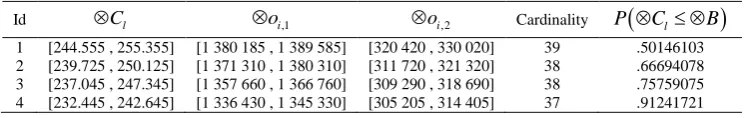
(30) Table 1 shows a few non-dominated solutions of Problem (28) for different  - values. More conservative (uncertainty averse) decision makers prefer a greater support.

[image:12.595.124.497.386.445.2]

The portfolios with Id = 1, 2, 3, 4 correspond to



0.5,0.66,0.75 and 0.9respectively. Taking into account that the available budget is estimated in the interval 240, 260, the first solution is very risky and the fourth solution seems to be very conservative. Let us suppose that the DM prefers solutions with



0.66 and



0.75.

Table 1. Some Pareto grey portfolios with different  values in Equation 40.

Id C_l o_i,1 oi,2 Cardinality P



  Cl B



113

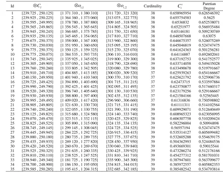
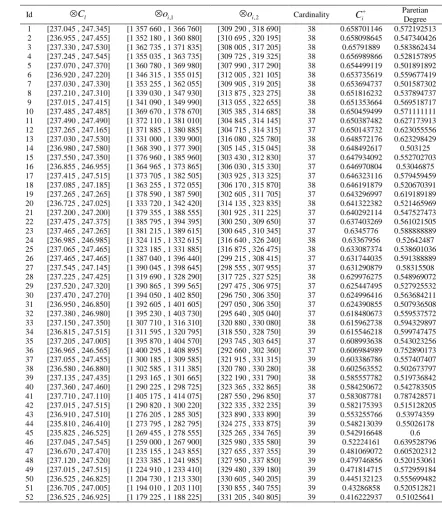
[image:13.595.61.510.92.437.2]

Table 2 shows the first front of the grey NSGA-II with



0.66 in Equation 40. The DM-decision analyst couple should choose the best compromise as a trade-off between the TOPSIS-Grey distance rank and the Paretian degree. This compromise should be in accordance with the DM’s attitude toward uncertainty. The solutions with Id=1 and Id=3 are good compromises. Table 3 shows results with a more level of conservatism (



0.75in Equation 40). The solution with Id=11 seems to be a good compromise.

Table 2. Results by TOPSIS-Grey method with



0.66(The budget is shown in million dollars).

Id Cl oi,1 oi,2 Cardinality Ci

 Paretian

114

The solution coming from Table 3 is a little more robust, but the compromise solutions from Table 2 have a bit better objective values. The DM-analyst couple has obtained the information necessary for making a final decision.

5.4.Comparison of results against a heuristic of the worst-case.

In this Section the term worst-case is introduced to refer a very conservative attitude of the DM, with the aim to perform a comparison between a worst-case experimentation and the results obtained in Section 5.2 in Tables 2 and 3. The worst-case attitude is reflected in resources and dominance, as described below:

(i) Resources: All the projects included in the portfolio consume the maximum costci, and the available budget is considered in its minimum level

 

B . Therefore, the constraint is defined as

1 * N

l i i i

C 



_c x B.

(ii) Dominance of worst-case between two grey vectors: Let D and E be two grey vectors; we say that D dominate E

[image:14.595.79.522.100.608.2]

 in the worst-case; if d_ie_i for all i values and there is at least one i such thatd_i e_i.

Table 3. Results by TOPSIS-Grey method with



0.75 (The budget is shown in million dollars).

Id C_l o_i,1 oi,2 Cardinality Ci

 Paretian

115

Experiments to find the worst-case in resources and dominance were carried out using the Algorithm 1, described in Section 4.1 but replacing the method of line 2 (which is responsible for generating the non-dominated fronts) with the Algorithm 4, which is shown.

With this replacement Algorithm 4 looks for solutions that are feasible and non-dominated in the worst case.

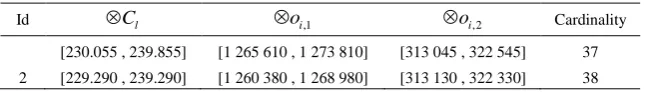
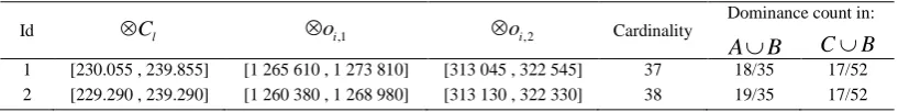
The experimental conditions are the same as described in Section 5.The solutions were obtained from 30 independent runs, generating two solutions whose values of budget, objectives, and cardinality are shown in Table 4.

[image:15.595.154.477.548.594.2]

To validate the solutions from our proposal, we gather the 35 solutions of Table 2 obtained with



0.66

 

 to 2 solutions obtained from the analysis of the worst-case

 

B . In the same way, we combine the solutions presented in Table 3 obtained with



0.75

 

C , with the set B.

Table 4. Solutions of the worst-case attitude reflected in resources and dominance.

Id C_l o_i,1 o_i,2 Cardinality

[230.055 , 239.855] [1 265 610 , 1 273 810] [313 045 , 322 545] 37

2 [229.290 , 239.290] [1 260 380 , 1 268 980] [313 130 , 322 330] 38

Algorithm 4. Worst-case-sort

 

P

1:for each  p P

2: dc_p 0

3: for each  q P

4: if



q p



then if q dominates pin the worst-case 5: dcpdcp1 Increment the domination counter of p

6:min=find-minimum

 

dc_p Minimum of the worst-case dominance count in P 7:cont=0

8:for each  p P

9: if dcpmin then p belongs to the first front

10: F₀ F₀ 

 

p

11: cont=cont+1

12: i=1 Initialize the front counter 13:while contP

14: Q  Used to store the members of the next front 15: for each  p P

16: min=min+1

17: if dcpmin then p belongs to the next front

18: Q  Q

 

p

19: cont=cont+1 20: i=i+1

116

By carrying out a dominance analysis in the set AB we obtained that all solutions in A continue being non-dominated, while the solutions of the worst-case B are dominated by many solutions of the setA.Something similar happens when the

dominance analysis is performed in the set



CB



; the solutions in C remain non-dominated in



CB



, while the solutions in B are dominated by many solutions inC

.

This is a consequence of the conservative handling of resource constraints under a worst-case attitude. Table 5 shows again the solutions of the setB, but now providing their dominance count when B is combined with A andC.

6. Conclusions.

This paper has presented a novel tool for describing and representing uncertainty associated with real-life decision-making problems. The problem of project portfolio selection was studied using mathematical modelling with the grey approach and considering relevant constraints, preferences, uncertainty and imprecision in the attributes such as project costs and scores as well as the total resources available.

The main contributions of this research are:

(i) Generalization of some basic concepts of multi-objective optimization to grey environment. (ii) Generalization of NSGA-II adapted to grey numbers.

(iii) Treatment of uncertainty in the project portfolio problem through grey mathematics. In particular, the ability to adjust the level of conservatism through the use of the support  and the Paretian degree.

The final solution is a compromise that involves DM preferences and beliefs combined with a robustness analysis. According to his/her particular beliefs and attitude toward uncertainty, firstly the DM should adjust the level of support related to the fulfillment of the total budget constraints. Once the approximation to the grey Pareto frontier has been obtained, the DM-decision analyst couple should select the best compromise considering the TOPSIS-Grey distance to the ideal solution and the Paretian degree.

In computer experiments our proposal gives evidence of good compromise solutions obtained as a function of our measures of quality and robustness.

Acknowledgements

We acknowledge support from PRODEP, Tecnológico Nacional de México and CONACyT (Fronteras de la Ciencia 2015-2 Proyecto: 1340, and Project 2015-280081 from the program Redes Temáticas Conacyt.)

References

1. Alvisi, S., Bernini, A., Franchini, M. A conceptual grey rainfall-runoff model for simulation with uncertainty. Journal Of Hydroinformatics, 15(1) (2013) 1-20.

2. Arasteh, A., Aliahmadi, A., Omran, M. M. Application of gray systems and fuzzy sets in combination with real options theory in project portfolio management. Arabian Journal for Science and Engineering, 39(8) (2014) 6489-6506.

3. Badri, M.A., Davis, D., Davis, D. A comprehensive 0-1 goal programming model for project selection. International Journal of Project Management, 19 (2001) 243-252. [4] Bhattacharyya, R., Kumar, P., Kar, S. Fuzzy R&D portfolio selection on interdependent projects. Computers and Mathematics with Applications, 62 (10) (2011) 3857-3870.

5. Carlsson, Ch., Fuller, R., Heikkila, M., Majlender, P. A fuzzy approach to R&D portfolio selection. International Journal of Approximate Reasoning, 44 (2) (2007) 93-105.

6. Coffin, M.A, Taylor, B.W. Multiple criteria R&D project selection and scheduling using fuzzy sets. Computers & Operations Research, 23 (3) (1996) 207-220.

[image:16.595.89.498.120.171.2]

7. Cruz-Reyes, L., Fernandez, E., Olmedo, R., Sanchez, P., Navarro, J. Preference Incorporation into evolutionary multiobjective optimization using preference information implicit in a set of assignment examples. In Fourth International Workshop on Knowledge Discovery, Knowledge Management and Decision Support. Atlantis Press, (2013) 179-187.

Table 5. Dominance count of solutions in the set B.

Id C_l o_i,1 oi,2 Cardinality

Dominance count in:

AB CB

117

8. Cruz-Reyes, L., Fernandez, E., Gomez, C., Sanchez, P. Preference Incorporation into Evolutionary Multiobjective Optimization Using a Multi-Criteria Evaluation Method. In Recent Advances on Hybrid Approaches for Designing Intelligent Systems. Springer International Publishing, (2014) 533-542.

9. Damghani, K.K., Sadi-Nezhad, S., Aryanezhad, M.B. A modular Decision Support System for optimum investment selection in presence of uncertainty: Combination of fuzzy mathematical programming and fuzzy rule based system. Expert Systems with Applications, 38(1) (2011) 824-834.

10. Deb, K., Agrawal, S., Pratap, A., Meyarivan, T. A fast elitist non-dominated sorting genetic algorithm for multi-objective optimization: NSGA-II. Lecture notes in computer science, 1917 (2000) 849-858.

11. Deb, K., Pratap, A., Agarwal, S., Meyarivan, T. A. M. T. A fast and elitist multiobjective genetic algorithm: NSGA-II. Evolutionary Computation, IEEE Transactions on, 6(2) (2002) 182-197.

12. Deb, K., Kumar, A. Interactive evolutionary multi-objective optimization and decision-making using reference direction method. In Proceedings of the 9th annual conference on Genetic and evolutionary computation, (2007) 781-788. ACM.

13. Deng, J.L. Control problems of grey systems. Systems & Control Letters, 1(5) (1982) 288-94.

14. Dickinson, M.W., Thornton, A.C., Graves, S. Technology portfolio management: Optimizing interdependent projects on multiple time periods. IEEE Transactions on Engineering Management, 48 (4) (2001) 518-527.

15. Duan, L., Duan, G. M., Lu, Q., Duan, J., XIE, L. Y., MU, Y. The status of traditional medicine and national medicine in different areas of the China in 2011 with grey clustering analysis. Grey Systems: Theory and Application, 4(2) (2014) 273-286.

16. Fernandez, E., Lopez, E., Bernal, S., Coello, C., Navarro, J., Evolutionary multiobjective optimization using an outranking-based dominance generalization. Computers & Operations Research, 37(2) (2010) 390-395.

17. Fernandez, E., Lopez, E., Lopez, F., Coello, C. Increasing selective pressure toward the best compromise in Evolutionary Multiobjective Optimization: the extended NOSGA method. Information Sciences, 181 (1) (2011) 44-56.

18. Fliedner, T., & Liesiö, J. Adjustable robustness for multi-attribute project portfolio selection. European Journal of Operational Research, 252(3) (2016) 931-946.

19. Huang, X. Optimal project selection with random fuzzy parameters. International Journal of Production Economics, , 106(2) (2007) 513-529.

20. Hwang, C.L., K. Yoon. Multiple Attribute Decision Making: Methods and Applications, (1981), Springer, Berlin, Heidelberg, New York.

21. Ji Shukla, O., Soni, G., Anand, G. An application of grey based decision making approach for the selection of manufacturing system. Grey Systems: Theory and Application, 4(3) (2014) 447-462.

22. Kleinmuntz, D. Portfolio Decision Analysis: Improved methods for resource allocation, chapter Foreword, Springer, New York-Dordrecht-Heidelberg-London, (2011) 5-7.

23. Klapka, J., Pinos, P. Decision support system for multicriterial R&D and information systems projects selection. European Journal of Operational Research, 140 (2) (2002) 434-446.

24. Kuchta, D. Use of fuzzy numbers in project risk (criticality) assessment. International Journal of Project Management, 19(5) (2001) 305-310.

25. Li, M., Jin, L., Wang, J. A new MCDM method combining QFD with TOPSIS for knowledge management system selection from the user's perspective in intuitionistic fuzzy environment. Applied soft computing, 21 (2014) 28-37.

26. Liesiö, J., Mild, P., Salo, A. Preference programming for robust portfolio modeling and project selection. European Journal of Operational Research, (2007), 181(3), 1488-1505.

27. Liesiö, J., Mild, P., Salo, A. Robust portfolio modeling with incomplete cost information and project interdependencies. European Journal of Operational Research, (2008), 190(3), 679-695.

28. Lin, Ch., Hsieh, P. A fuzzy decision support system for strategic portfolio management. Decision Support Systems, 38(3) (2004) 383-398.

29. Lin, Y. H., Lee, P. C., Ting, H. I. Dynamic multi-attribute decision making model with grey number evaluations. Expert Systems with Applications, 35(4) (2008) 1638-1644.

30. Liu, S., Lin, Y., Forrest, J. Y. L. Grey systems: theory and applications. Springer Science & Business Media. 68 (2010) 31. Luo, D., Li, Y. Multi-stage and multi-attribute risk group decision-making method based on grey information. Grey Systems:

Theory and Application, 5(2) (2015) 222-233.

32. Moore, R.E.: Interval arithmetic and automatic error analysis in digital computing. Ph. D. Dissertation, Department of Mathematics, Stanford University, Stanford, CA (1962)

33. Radulescu, C.Z., Radulescu, M. Project portfolio selection models and decision support. Studies in Informatics and Control, 10 (4) (2001) 275-286.

34. Rabbani, M., Aramoon, M., Baharian, G. A multi-objective particle swarm optimization for project selection problem. Expert Systems with Applications, 37(1) (2010) 315-321.

35. Ringuest, J. L., Graves, S. B., Case, R. H. Mean–Gini analysis in R&D portfolio selection. European Journal of Operational Research, 154(1) (2004) 157-169.

36. Rivera, G., Cruz, L., Fernandez, E., Gomez, C., Perez, F. Many-objective portfolio optimization of interdependent projects with ‘a priori’incorporation of decision-maker preferences. Appl. Math, 8(4) (2014) 1517-1531.

37. Roy, B. Robustness for Operations Research and Decision Aiding. (2013) <hal-00874341>

38. Salo, A., Keisler, J., Morton, A. Portfolio Decision Analysis. Improved methods for resource allocation, International Series in Operations Research & Management Science, chapter An invitation to Portfolio Decision Analysis. Springer New York, 162 (2011) 3-27.

39. Santhanam, R., Kyparisis, J. A multiple criteria decision model for information system project selection. Computers and Operations Research, 22-8 (1995) 807-818.

40. Sadeghi, M., Hajiagha, S. H. R., Hashemi, S. S. A fuzzy grey goal programming approach for aggregate production planning. The International Journal of Advanced Manufacturing Technology, 64(9-12) (2013) 1715-1727.

118

42. Shih, H. S., Shyur, H. J., Lee, E. S. An extension of TOPSIS for group decision making. Mathematical and Computer Modelling, 45(7) (2007) 801-813.

43. Stummer, C., Heidemberger, K. Interactive R&D portfolio analysis with project interdependencies and time profiles of multiple objectives. IEEE Transactions on Engineering Management, 30 (2) (2003) 175-183.

44. Sunaga, T.: Theory of interval algebra and its application to numerical analysis. RAAG Memoires 2, (1958)
29–46.

45. Yan, X. Z., Song, Z. M. The portfolio models of contained grey profit under uncertainty. Grey Systems: Theory and Application, 4(3) (2014) 487-494.

46. Yang, Y., Yang, S., Ma, Y. A literature review on decision making approaches for research and development project portfolio selection (2012).