Empirical Analysis of Regional Financial Development and Regional Economic Growth—Based on the Data of Fifteen States in Xinjiang

(1)

http://www.scirp.org/journal/jfrm ISSN Online: 2167-9541

ISSN Print: 2167-9533

DOI: 10.4236/jfrm.2017.64029 Dec. 27, 2017 397 Journal of Financial Risk Management

Empirical Analysis of Regional Financial

Development and Regional Economic Growth

—Based on the Data of Fifteen States in Xinjiang

Xu Si

School of Economics, Jinan University, Guangzhou, China

Abstract

This article collected panel data of fifteen states of Xinjiang between 2005 and 2011, and based on the method of quantile regression, made an empirical re-search among financial development and economic growth of Xinjiang fifteen states. The financial related rate, the efficiency of financial intermediation, the structure of financial savings and insurance depth were included in this paper. Conclusion: Comprehensive financial development level (LNFIR, LNFAE, LNFSS, LNIND) in different quantile level factor of economic growth, region-al financiregion-al development level of Xinjiang restricts economic growth. Finregion-ally, this paper, according to the empirical results, puts forward the “financial de-velopment cycle theory”, and puts forward some suggestions.

Keywords

Xinjiang Fifteen States, Financial Development, Economic Growth, Quantile Regression

1. Introduction

In the third Plenary Session of the 16th_{CPC (Communist Party of China)} Cen-tral Committee, China put forward the Scientific Outlook on Development problem, its content is comprehensive, coordinated and sustainable develop-ment. Therefore, from the perspective of sustainable development of regional economy, it is necessary to study the relationship between financial development and economic growth in a region. In recent years, the world situation has un-dergone profound changes, and China’s development is still in an important pe-riod of strategic opportunities, is facing a rare historical opportunity, but also facing many predictable and unpredictable risks and challenges. In order to seize How to cite this paper: Si, X. (2017).

Em-pirical Analysis of Regional Financial De-velopment and Regional Economic Growth. Journal of Financial Risk Management, 6, 397-417.

https://doi.org/10.4236/jfrm.2017.64029

Received: November 30, 2017 Accepted: December 24, 2017 Published: December 27, 2017

http://creativecommons.org/licenses/by/4.0/

(2)

DOI: 10.4236/jfrm.2017.64029 398 Journal of Financial Risk Management the opportunity to deal with the challenge, the “12th Five-Year” plan is intro-duced in a timely manner. During the “12th Five-Year”, the government put the strategy on the implementation of the western development strategy in the over-all strategic priority of regional development. We should give full play to the comparative advantages of all regions, promote the rational flow of regional production factors and orderly transfer of industries, and cultivate new regional economic growth poles in the Midwest. Xinjiang economic work conference has been held, nineteen provinces and cities Yuanjiang work in full swing, the prefe-rential policies for Xinjiang have been introduced, which undoubtedly made an unprecedented foreshadowing for the regional economic development

2. Literature Review

(3)

DOI: 10.4236/jfrm.2017.64029 399 Journal of Financial Risk Management foreign economists has been more mature. For instance, Levine (1997), Becker-man (1998). At present, most of the foreign scholars think that the economic and financial influence each other, unfortunately, but they can not give a stan-dard conclusion.

In our country, The research on the relationship between regional financial development and regional economic growth have not formed a theoretical sys-tem, most of them nearly indiscriminately imitate the western theory, and all of our scholars verify the existing western theory by use different methods or in different period or based on different data, innovative thinking is very lack. Of course, it also has some significance. Liu (2002) made a simple linear regression using the average cross sectional data of 31 provinces (autonomous regions and municipalities directly under the central government) in mainland China for three years in 1998-2000 years. But because of the simple linear regression, the probability of error is higher, so the result is very unreliable. Zhou and Zhong (2004) studied the relationship between financial development and economic growth based on the data of China’s central, western and eastern. Results showed that financial development and economic growth has formed a benign interaction in the eastern, while in the west, this interaction has not yet ap-peared. Wang (2005) analyzed the whole data of eastern and western during the period 1990-2002, his conclusion is that there exists long-term cointegration re-lationship between the eastern and western regions of financial development and economic growth, and financial development has obvious promotion effect on economic growth in eastern, but there is a mutual inhibition relationship be-tween financial development and economic growth in the West. Ma (2006) use the granger-causality test respectively on the 1980-2000 data of Eastern, central and Western verification shows that significant reciprocal causation relationship exists between the eastern and central economic growth and financial develop-ment, economic growth in the western region has significantly promoted the development of finance, financial development has a certain role in promoting economic growth, but effect is not obvious, similar results are also obtained, such as Ran (2006), Xu (2007), etc. The more objective research comes from Wu (2009, 2010), his analysis based on quantile regression, show that financial de-velopment on the impact of economic growth and volatility is statistically signif-icant in different quantiles of economic growth. But there’s nothing new about it. Therefore, to sum up, we know that the study of regional economic growth and financial development by scholars in China remains at the level of verifica-tion of the existing theories in the west.

3. Empirical Analysis of Regional Financial Development

and Regional Economic Growth

3.1. Object Description, Model Setting and Data Source

(4)

DOI: 10.4236/jfrm.2017.64029 400 Journal of Financial Risk Management planning of the main functional areas of Xinjiang is as follows: Urumqi, Kara-may, Shihezi, Turpan area, Hami area, Changji area, Yili aera, Tacheng aera, Aletai aera area, Bazhou, Bozhou, Akesu, Kashi area, Hetian area, Altai moun-tain forest ecological function area, the Tarim River desert ecological function area, Altun Mountains grassland ecological function zone. Taking into account the specific situation of each functional area, the state of Yili directly under the county expanded to Yili state, so this paper chooses Urumqi, Karamay, Shihezi, Yili area, Turpan area, Hami area, Changji area, Tacheng area, Aletai area, Boz-hou, BazBoz-hou, Akesu area, Kashi area, Hetian area, total of fifteen states. We im-plement an empirical analysis for the relationship between financial develop-ment and economic growth in the fifteen states based on the method of quantile regression. In order to maintain the consistency of statistical indicators, the data in our study from the fifteen prefectures of Xinjiang “national economic and so-cial development statistics bulletin 2005-2011”, and “Xinjiang Statistical Year-book 2006-2012”, the actual time of data is 2005-2011 (detailed data are shown in the appendix). What needs to be explained is that: some of missing values and outlier, we use the method for making up missing values in time series to com-plement missing values and replace the outlier.

In the empirical literature of economic growth, production function is a basic estimation framework. In our empirical research, we also use it to analysis the relationship between regional financial development and economic growth, set the total production function (T) in the form of the output as a function of the abstract level of financial development and control variables, control variables are other main factors in addition to the variables thus describe the financial de-velopment level, so it can be expressed as:

(

Finance , Controltt t

)

t

Y =F

(1)

Notes: Yt represents output or added value, it is generally replaced by GDP;

t

Finance is the level of financial development; Controlt is the control variable.

Generally, if the elasticity research is carried out, it can be expanded on the basis of Cobb Douglas type production function. Based on the available data re-search the relationship between financial development and economic growth of Xinjiang’s fifteen prefectures. The explained variable take per capita GDP re-flects the economic growth, with GDPP representation; explanatory variables takes two groups of variables: the financial development level and control va-riables. They are defined as follows:

1) The level of financial development

Financial related ratio: FIR = Financial institutions loans/GDP Financial intermediation efficiency: FAE = Loan/Deposit Financial savings structure: FSS = Savings/All deposits Insurance depth: IND = Premium income/GDP 2) Control variable

Physical capital input: GTZB = Region total fixed capital/GDP

(5)

DOI: 10.4236/jfrm.2017.64029 401 Journal of Financial Risk Management Economic openness degree:

CKZB

= Total export trade/GDP

Labor input: LDZB = Total wages of staff and workers/

GDP

According to the above discussion, we need to carry out the elasticity research, the model is set as follows:

0 1 2 3 4

5 6 7 8

t t t t t

LnGDPP LnGTZB LnCZZB LnCKZB LnLDZB

LnFIR LnFAE LnFSS LnIND

β β β β β

β β β β µ

= + ∗ + ∗ + ∗ + ∗

+ ∗ + ∗ + ∗ + ∗ + (2)

3.2. Fifteen Prefectures of Xinjiang Financial Development and

Economic Growth: Conditional Quantile Regression Results

and Statistical Analysis

3.2.1. Comparison of Estimation Results between Conditional Median Regression and Conditional Mean Regression

2005-2011 in fifteen prefectures of Xinjiang financial development and econom-ic growth data, including a total of 105 groups of sample data of 15 states in 7 years, relatively large sample. For comparison, conditional median regression and conditional mean regression were used for empirical analysis. This paper focuses on the similarities and differences between estimation methods, statistic-al tests (goodness of fit, equation significance test, significance test of variables) and the estimation of equation coefficients.

1) Estimation method

The results of conditional median regression are shown in Table 1, and the results of conditional mean regression are shown in Table 2. The estimation me-thod of conditional quantile (median) regression and conditional mean regression is different, the conditional quantile (median) use Least absolute-deviations (LAD) estimator to estimate, the conditional mean regression use Leat squares devia-tions (LSD) estimator to estimate. Therefore, the estimation results are naturally different due to the different estimation methods.

2) Statistical test

The significance test (Quasi-LR test and F test) of conditional median regres-sion and conditional mean regresregres-sion were statistically significant at the signifi-cant level of 0.01. Variable significance test (t-test), in addition to the variables in Table 1, LNCKZB, LNLDZB and Table 2, the variable LNCKZB is not statisti-cally significant at the significant level of 0.10, other variables in Table 1 and Table 2 are statistically significant at the significant level of 0.05. Because of the different calculation methods, the goodness of fit of the two estimation methods is obviously different. Generally, based on the same data, the pseudo goodness of fit (Pseudo R-squared) was significantly smaller than the goodness of fit (R-squared), and the adjusted pseudo goodness of fit (Adjusted Pseudo R-squared) was sig-nificantly smaller than the adjusted goodness of fit (Adjusted R-squared). In Ta-ble 1, Pseudo R-squared = 0.6182, Adjusted Pseudo R-squared=0.5864; In Table 2, R-squared = 0.8366, Adjusted R-squared=0.8230. In addition, in Table 2, D.W = 0.6636, because D.W. = 2 (1 −

ρ

_{), can calculate the}

ρ

_{= 0.6682, showed a}

(6)

[image:6.595.208.539.88.363.2]

DOI: 10.4236/jfrm.2017.64029 402 Journal of Financial Risk Management

Table 1. Conditional median regression results.

Variable Coefficient Std. Error t-Statistic Prob. C 11.20185 0.987134 11.34785 0.0000 LNGTZB 0.85292 0.172232 4.952158 0.0000 LNCZZB −0.634153 0.123479 −5.135692 0.0000 LNCKZB 0.015274 0.03691 0.413809 0.6799 LNLDZB −0.343962 0.286338 −1.201246 0.2326 LNFIR −1.161545 0.283865 −4.091887 0.0001 LNFAE 1.373073 0.471864 2.909892 0.0045 LNFSS −2.166223 0.419899 −5.158918 0.0000 LNIND 0.965763 0.224689 4.298218 0.0000 Pseudo R-squared 0.618192 Mean dependent var 9.825069 Adjusted R-squared 0.586374 S.D. dependent var 0.870102 S.E. of regression 0.385351 Objective 13.53921 Quantile dependent var 9.923045 Objective (const. only) 35.46077 Sparsity 0.861560 Quasi−LR statistic 203.5521 Prob(Quasi-LR stat) 0.000000

Note: 1) Dependent Variable: LNGDPP; 2) Method: Quantile Regression (Median); 3) Sample: 2005-2011; 4) Bootstrap method: XY-pair, reps = 200, mg = kn, seed = 673,929,944; 5) Included observations: 609.

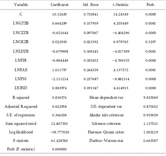
Table 2. Conditional mean regression results.

[image:6.595.209.540.417.728.2]

(7)

DOI: 10.4236/jfrm.2017.64029 403 Journal of Financial Risk Management R-squared and Adjusted R-squared have exceeded 0.80. Furthermore, there was no sequence correlation test for conditional median regression in Table 1, in order to increase the comparability, the conditional mean reversion with AR (1) is no longer given in this paper.

3) Equation coefficient estimation

The values of the conditional median regression estimator and the conditional mean regression estimator of the corresponding coefficients are obviously dif-ferent. However, there is no change in the conditional median regression esti-mator corresponding to the eight explanatory variable coefficients and the sym-bol of conditional mean regression estimator. In the conditional median regres-sion model, the estimation values of LNCKZB and LNLDZB were not significant in T-test, the rest are significant; in the conditional mean regression model, the estimation of LNCKZB is not significant, others are significant. In the condi-tional median regression model, the absolute value of the estimated variables LNCKZB and LNLDZB coefficients is less than the absolute value of the esti-mated value of the conditional mean regression explanatory variable coefficient; The absolute values of the explanatory variables LNGTZB, LNCZZB, LNFIR, LNFAE, LNFSS and LNIND coefficients in the conditional median regression model are greater than the absolute values of the estimated values of the condi-tional mean regression explanatory variable coefficients.

3.2.2. Analysis of the Difference and Variation of Conditional Quantile Regression Estimation Coefficients

As mentioned before, as a result of the economic gap between the various pre-fectures of Xinjiang, the Xinjiang economic development empirical analysis, put forward the countermeasures, it can not be generalized, not the statistical regres-sion analysis using traditional statistical methods for the average properties. Quantile regression analysis can solve this problem. As mentioned before, be-cause the regional economic disparity is obvious in all aspects of Xinjiang, therefore, an empirical analysis of Xinjiang’s economic development and put forward the countermeasures, we can not generalize, the traditional statistical methods can not be used for the regression analysis of the average properties. quantile regression analysis can solve this problem.

(8)

[image:8.595.209.537.91.720.2]

Table 3. Quantile regression coefficient result.

(9)

DOI: 10.4236/jfrm.2017.64029 405 Journal of Financial Risk Management Continued

0.3 −2.472365 0.294652 −8.390783 0.0000 0.5 −2.166223 0.419899 −5.158918 0.0000 0.7 −1.745039 0.376772 −4.631555 0.0000 0.9 −2.307105 0.631270 −3.654703 0.0004 LNIND 0.1 1.239505 0.409374 3.027807 0.0032 0.3 1.201106 0.268524 4.472999 0.0000 0.5 0.965763 0.224689 4.298218 0.0000 0.7 0.892971 0.216263 4.129106 0.0001 0.9 0.962809 0.376418 2.557820 0.0121

1) The difference analysis of the estimators of the coefficients of different ex-planatory variables. In a specific quantile level of economic growth, the impact of financial development and other control variables on economic growth is dif-ferent. Specifically, as shown in Table 3, the coefficients of the explanatory va-riables, LNGTZB, LNFAE, and LNIND, are positive in the different quantile le-vels of the explained variable LNGDPP, the coefficients of the explanatory va-riables LNCZZB, LNLDZB, LNFIR and LNFSS are negative, and the absolute value of the coefficient of the variable LNFSS is the largest at all the quantiles. The coefficient of explanatory variable LNCKZB is negative at the 0.1 and 0.9 quantiles of the explained variable. It is positive at other quantiles, and the abso-lute value of the negative coefficient is larger than the positive value, but its ab-solute value is the smallest compared with other variables. In addition, it is easy to see that the standard deviation of the quantile regression coefficient obtained by the repeated sampling of the self-help method (bootstrap) is also different from the standard deviation of the quantile regression coefficient obtained by the 200 times. For every specific quantile level of economic growth, the standard deviation of the coefficient of explanatory variable LNCKZB is the smallest, while the standard deviation of the coefficients of explanatory variables LNFAE and LNFSS is relatively large. In addition, the standard deviation of regression coefficient near the 0.5 quantile is relatively small, and the standard deviation of regression coefficient near the 0.1 and 0.9 percentile is relatively large. Notabili-ty, the tail probabilities of the significance test of the regression coefficient of the explanatory variable LNCKZB near the quantiles were more than 0.10, The tail probabilities of the significance test of the regression coefficient at the 0.1, 0.3, and 0.5 quantiles of the explanatory variable LNLDZB are all greater than 0.10. Only the P value of the tail probability of the LNFAE variable in the 0.1 and 0.9 quantile regression coefficient significant test appears more than 0.10. the top down is 0.2556 and 0.1636, respectively.

(10)

DOI: 10.4236/jfrm.2017.64029 406 Journal of Financial Risk Management LNGDPP increases from 0.1 to 0.9. The point estimates for the coefficients of the explanatory variables (financial development and other control variables) are all changing. We focus on the analysis of the variation characteristics of the coeffi-cient points of the variables related to the level of financial development. That is, the explanatory variables LNFIR, LNFAE, LNFSS, LNIND, specifically expressed as: The coefficient of the explanatory variable LNFIR is reduced first and then incrementing, the coefficient of LNFIR begins to increase from the 0.30 digits of LNGDPP, it basically reflects the basic law of the loan function of financial in-stitutions with different quantile levels in LNGDPP of fifteen prefectures of Xin-jiang; The coefficient of LNFAE increasing first and then decreasing, basically, the coefficient of LNFAE begins to become smaller at the 0.30 digits of the in-terpreted variable LNGDPP, it basically reflects the basic law of efficiency of fi-nancial intermediary role with different quantile levels in LNGDPP of fifteen prefectures of Xinjiang; The coefficient of the explanatory variable LNFSS has two sharp drops at both ends, it is gradually smaller from 0.1 to 0.3 quantiles of LNGDPP, from 0.3 to 0.7, it is progressively larger, from 0.7 to 0.9, the number is gradually reduced, This basically reflects the basic law of financial savings structure; The coefficient of the explanatory variable LNIND is reduced first and then incrementing, the coefficient of LNIND began to increase at At the 0.7 per-centile of LNGDPP, which basically reflects the basic rules of the insurance in-dustry.

4. Conclusions and Policy Recommendations

4.1. Conclusion

(11)

DOI: 10.4236/jfrm.2017.64029 407 Journal of Financial Risk Management economic growth, financial development will restrict economic growth or there is no relationship between financial development and economic growth is one- sided. From the data analysis results, we can see that in different stages of eco-nomic development, the level of financial development plays a different role in economic growth, and the extent of action is also different. That is, in the “bud-ding period” of finance, economic growth needs to nurture financial develop-ment, at this time, financial development needs compensation from other sec-tors of the economy, at this stage, finance is a drag on economic growth; To the “growth period” of finance, financial development and economic growth are coordinated and mutually promoting, in this stage, if the two are not coordi-nated, there will be mutual constraints, but it is often difficult to coordinate the development of the two; If the financial level continues to develop, it will enter the “mature period”, financial development will serve the economic growth well; If finance continues to develop and enter the “period of excessive prosperity”, financial development will be a factor that restricts economic growth, and even lead to a recession and the collapse of the financial system, for example, Wall Street and Wenzhou folk lending.

4.2. Policy Recommendations

4.2.1. Efforts to Promote Leapfrog Development of Financial Scale and Efficiency with the Aid of Policy

Our state has paid more and more attention to the economic development of Xinjiang, and has launched a new round of support for Xinjiang. This provides an unprecedented opportunity for Xinjiang’s economic development. Chiefly, Xinjiang fifteen prefectures need to clear their own financial development stage, From the financial related ratio (FIR), the loans of Urumqi and Shihezi are more than its GDP, the rest are less than 1, mostly in 0.4 - 0.6, the lowest is Karamay, the financial related ratio is 0.17. Reference to Appendix Table A11. But there is no doubt that Urumqi and Karamay are the richest areas in Xinjiang, which means Urumqi relies on the total financial volume, while Karamay wins by the financial benefit (the paper defined as the gains from the financial assets of the unit). It is pointed out the development direction for other states in Xinjiang, For example, Shihezi, Hami, and Kashi with higher financial related ratios(FIR), they can continue to expand the financial scale, improve the financial related tio and realize the leapfrog development. States with lower financial related ra-tios should be to expand the scale of the finance, at the same time, more efforts should be made in the financial efficiency, and the national wealth, supported by the unit loans, is constantly increasing, and the financial benefits are constantly improved, and the leap forward development is finally achieved.

4.2.2. Vigorously Advocates the Spirit of Contract, Optimizes the Environment of Indirect Financing, and Improves

the Efficiency of Financial Intermediation (FAE)

(12)

DOI: 10.4236/jfrm.2017.64029 408 Journal of Financial Risk Management is still high, the construction of various laws and regulations is more serious and more complicated. But the modern economic society is in the era of contract economy, without the spirit of contract, it is hard for the society to have a good faith environment and lack of integrity. As a core of indirect financing business, banks will inevitably raise the loan threshold. As a result, enterprises or individ-uals who are short of money can hardly get the support needed, which hinders the development of enterprises and individuals, and can not provide enough power for economic growth. From the empirical results, we can see that the effi-ciency of financial intermediation has a significant positive impact on economic growth at each quantiles. In fact, The efficiency of financial intermediation in fifteen prefectures of Xinjiang mostly in the 30% - 55% level, no area reached the level of 70%, details see Appendix Table A12. Therefore, Xinjiang fifteen pre-fectures should vigorously promote the spirit of contract, to optimize the indi-rect financing environment, even the implementation of the national rural bank lending patterns—Five household joint insurance, and actively establish the lin-kage mechanism between finance, prompting banks to reduce lending threshold, in order to improve the efficiency of financial intermediation, so as to promote the regional economic growth.

4.2.3. Speed up the Establishment and Improvement of Social Security System, Reduce the Saving Levels

Macroeconomics believes that savings can provide the funds needed for eco-nomic growth, however, if the social savings rate is generally high, residents have less disposable income to consume, and lack of consumption, that is, lack of de-mand, which will surely lead to slow economic growth or even zero growth. It can be seen from the empirical results of this article, Xinjiang’s state financial savings structure (LNFSS) has a significant negative impact on economic growth at all the quantile levels, and the absolute value of the influence coefficient on the economy is the largest at each quantiles, it can be seen that the financial savings structure in Xinjiang has been a serious impediment to economic growth. Therefore, the reduction of the social savings rate is to provide demand for the economic development. It’s easy to think that people’s high saving concept is only to cope with unexpected needs. If the social security system is perfect, people will consume (of course, do not encourage extravagance and waste), so that economic development will be strongly supported.

4.2.4. Widely Publicized Insurance Undertakings and Accelerated the Development of Insurance

(13)

DOI: 10.4236/jfrm.2017.64029 409 Journal of Financial Risk Management insurance, fear will be reduced or even disappear, therefore, to speed up the de-velopment of the insurance industry is very important. From the empirical re-sults, we can see that insurance depth (LNIND) has a significant positive impact on economic growth at all quantile levels, and also has a greater impact.

References

Beckerman, P. (1998). The Consequences of` Upward Financial Repression. Review of Radical Political Economics, 2, No. 1.

Goldsmith, R. W. (1969). Financial Structure and Development. New Haven, CT: Yale University Press.

Greenwood, J., & Jovanovic, B. (1990). Financial Development, Growth and the Distribu-tion of Income. Journal of Political Economy, 98, No. 5, Part 1.

https://doi.org/10.1086/261720

Krugman, P. (2003) The Myth of Asia’s Miracle. Foreign Affairs, 73, 62-78.

https://doi.org/10.2307/20046929

Levine, R. (1997). Financial Development and Economic Growth: Views and Agenda. Journal of Economic Literature, XXXV, 688-726.

Liu, X. R. (2002). An Empirical Analysis of the Relationship between Regional Financial Development and Economic Growth in China. Journal of Southwest National Acade-my of Nationalities, 12, 109-112.

Lucas, R. E. (1988). On the Mechanics of Economic Development. Journal of Monetary Economics, 22, 3-42.

Ma, R. Y. (2006). An Empirical Analysis of the Relationship between Regional Financial Development and Economic Growth in China. Finance Teaching and Research, 2, 2-5. McKinnon, R. I. (1973). Money and Capital in Economic Development. Washington, DC:

The Brookings Institution.

Patrick, H. T. (1966). Financial Development and Economic Growth in Underdeveloped Countries. Economic Development and Cultural Change, 14, 174.

https://doi.org/10.1086/450153

Ran, G. H. (2006). Regional Differences in the Relationship between Financial Develop-ment and Economic Growth in China—Based on the Test and Analysis of the Eastern and Western Panel Data. China Soft Science, 2, 102-110.

Schumpeter, J. (1911). The Theory of Economic Development: An Inquiry into Profits, Capital, Credit, Interest, and the Business Cycle. Cambridge, MA: Harvard University Press.

Shaw, E. S. (1973). Financial Deepening in Economic Development. New York: Oxford University Press.

Wang, J. W. (2005). Financial Development and Economic Growth: An Empirical Analy-sis Based on China’s Regional Financial Development, Finance and Trade Economics, 10, 23-26+96.

Wu, Y. Z. (2009). Empirical Analysis on Regional Financial Development and Economic Growth—Based on Prefecture Level City data of Ten Provinces in East China and Quantile Regression Method. Statistics Education, 3, 12-17.

(14)

DOI: 10.4236/jfrm.2017.64029 410 Journal of Financial Risk Management Xu, J. (2007). The Analysis of the Coordination of Regional Financial Development and Economic Growth—An Analysis of the Regional Impact of Macro Regulation. Finan-cial vertical and horizontal, 3, 32-34.

(15)

[image:15.595.208.539.108.379.2]

Appendix

Table A1. Gross domestic product (100 million yuan).

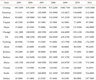
State 2005 2006 2007 2008 2009 2010 2011 Urumqi 562.5007 654.3023 820.2800 1020.3500 1087.5000 1338.5172 1700.0000 Karamay 385.7256 473.2562 515.1297 661.2100 480.2900 711.3532 800.0000 Shihezi 53.7455 61.8382 73.2468 90.9700 108.3600 134.9995 243.2700 Turpan 119.7738 148.2271 172.0268 201.2300 154.5800 182.7866 217.5000 Hami 68.5715 77.6355 91.9912 126.9000 130.3200 167.3848 217.8200 Changji 251.6925 295.9704 313.1995 388.1500 444.7100 557.9917 702.0000 Yili 373.0401 444.6349 539.6630 670.0900 735.8700 885.0339 1091.8400 Tacheng 143.9680 167.8464 203.9121 261.2100 284.8200 341.9047 353.3000

Aletai 60.5144 80.6145 99.2804 117.6500 117.3900 134.8644 162.9400 Bozhou 55.4598 63.1628 77.0414 88.2200 100.9600 131.4500 151.6000 Bazhou 325.6885 409.7582 469.0028 585.7600 525.9400 640.1378 800.0000 Akesu 170.4286 193.7736 231.5179 273.1200 320.4500 396.1175 778.7800 Tomsk 17.4718 19.7129 23.7132 27.6800 32.4600 38.8757 44.5516

Kashi 136.0000 183.2222 239.1600 238.5700 284.2400 359.9718 467.3000 Hetian 48.7832 55.3429 63.6962 74.5200 88.5800 103.4972 126.6300 Data source: Xinjiang fifteen prefectures “national economic and social development statistics bulletin 2005-2011”.

Table A2. Per capita gross domestic product (yuan).

State 2005 2006 2007 2008 2009 2010 2011 Urumqi 25,507 28,261 31,140 37,343 38,249 43,039 52,925 Karamay 88,562 96,006 98,398 100,216 87,000 121,387 211,529

Shihezi 17,854 20,395 23,797 29,073 34,421 42,816 38,961 Turpan 20,580 25,252 28,907 33,332 25,741 29,828 34,674 Hami 12,865 14,354 16,910 22,887 23,055 29,375 37,694 Changji 15,169 17,666 20,893 25,411 28,520 35,554 43,251 Yili 8759 10,345 12,349 15,054 16,221 19,479 23,790 Tacheng 11,113 12,872 15,451 19,587 20,784 23,562 26,719 Aletai 10,822 14,288 17,412 20,379 19,903 22,406 26,799 Bozhou 12,188 13,598 16,437 18,573 21,130 27,374 33,040 Bazhou 27,302 33,689 37,466 45,669 39,467 46,955 58,565 Akesu 7620 8471 9898 11,413 13,098 15,872 30,388 Tomsk 3654 4051 4712 5350 6183 7202 8476

[image:15.595.208.540.436.701.2]

(16)

[image:16.595.207.540.89.360.2]

Table A3. Total investment in fixed assets (billion yuan).

State 2005 2006 2007 2008 2009 2010 2011 Urumqi 220.2909 248.6804 315.0310 380.1799 598.0250 690.0569 635.0000 Karamay 134.5609 207.5271 286.1913 238.9397 186.6073 193.4056 209.6000 Shihezi 31.0157 35.5352 54.9008 60.6211 69.7916 102.3823 200.3600 Turpan 41.5629 55.7363 61.3575 81.5173 80.4752 94.3186 134.8000 Hami 17.0658 32.0458 39.7082 63.0731 95.6549 149.2069 307.8700 Changji 83.7217 111.4195 112.5342 141.9867 205.0815 298.8210 508.8000 Yili 151.3349 181.3077 194.0315 268.9166 395.5974 602.0137 734.1900 Tacheng 46.8332 57.4896 67.6355 83.8981 124.3716 187.8818 187.4000 Aletai 27.9728 31.2107 38.2171 55.2065 77.9338 112.3135 127.8400 Bozhou 16.5366 19.1529 26.4830 30.0290 47.2660 67.9162 74.3682 Bazhou 160.0939 195.2750 210.0681 249.3021 252.8522 310.2994 416.7000

Akesu 74.1326 104.4280 113.3263 106.9756 234.0250 181.6968 252.1000 Tomsk 9.4918 10.3283 12.1096 15.7207 27.3966 31.8417 46.3934

Table A4. Total financial expenditure (100 million yuan).

State 2005 2006 2007 2008 2009 2010 2011 Urumqi 41.6980 49.5342 68.3153 99.3534 163.5900 208.2300 299.7100 Karamay 28.4139 34.7690 42.8248 46.5476 42.7153 54.7711 70.8000

Shihezi 5.5033 6.8537 8.4440 10.9640 14.0114 17.2440 21.2224 Turpan 9.5549 13.3250 16.5740 22.9677 25.9159 33.2106 49.1000 Hami 10.1766 13.0768 16.3823 23.4935 29.3562 38.6270 58.8200 Changji 22.5949 30.8067 34.4146 49.7816 70.8200 98.6000 155.3900

Yili 68.9285 87.5453 113.4352 154.3933 199.2916 264.6054 396.6700 Tacheng 18.9016 25.4619 32.3630 42.9826 48.9470 68.5169 98.0300 Aletai 15.2517 18.7916 25.4934 36.7277 52.7425 67.8883 91.6800 Bozhou 9.3148 10.9711 15.3008 20.1823 24.9022 31.5170 44.1800 Bazhou 24.7944 31.9573 39.6809 55.3026 66.5735 88.0084 143.6000

Akesu 31.3866 40.8242 53.8450 74.6619 86.4291 114.3958 182.0300 Tomsk 11.2770 14.6184 17.8392 24.8689 33.8557 41.9683 43.8000

[image:16.595.208.539.417.696.2]

(17)

[image:17.595.208.539.89.360.2]

Table A5. Total export trade (100 million yuan).

Shihezi 8.4145 9.3848 17.2240 24.2103 11.4694 29.7708 53.5081 Turpan 0.0221 0.1515 0.2936 0.4217 0.6237 0.4414 1.5570

Hami 1.1112 3.5745 3.1060 3.4726 3.2837 1.1984 1.2748 Changji 58.2944 102.8693 174.9618 240.9685 131.6537 129.7784 125.7192

Yili 157.6445 177.0013 237.5507 482.7679 272.0301 285.4976 273.4807 Tacheng 35.2618 32.5080 56.9977 69.1924 56.1769 35.9678 16.8584

Aletai 1.6726 0.9465 2.9827 18.6304 31.5221 46.0536 55.3064 Bozhou 54.7428 61.2636 38.2561 53.5524 27.2848 24.4432 66.2294 Bazhou 1.5398 6.6204 18.0790 31.0548 5.9150 7.3215 6.5990

Akesu 0.3065 0.9010 1.5526 5.5772 9.2445 17.4047 20.0303 Tomsk 3.0264 5.0727 18.0326 19.4530 8.0382 3.6851 5.4759

Table A6. Total wages ($100 million).

[image:17.595.208.540.416.699.2]

(18)

[image:18.595.208.539.88.359.2]

Table A7. Deposit balance (100 million yuan).

State 2005 2006 2007 2008 2009 2010 2011 Urumqi 1410.0300 1685.5400 2056.0900 2371.9600 2935.1800 3596.4300 4080.5000 Karamay 231.9000 272.7000 285.9000 320.4800 489.9000 792.5000 860.8000 Shihezi 126.4700 144.5000 159.4500 185.8600 225.6400 296.2700 356.1900 Turpan 64.0100 76.5000 81.1000 82.2000 100.2000 131.3000 148.9000 Hami 115.2700 135.8200 148.0700 163.2600 193.2400 257.2900 316.0000 Changji 213.5900 247.0500 264.5900 322.4800 433.9000 562.3700 655.0200 Yili 402.2700 478.5500 533.5800 632.9600 789.7600 1019.6300 1251.7400 Tacheng 103.5400 116.5000 123.5400 147.9600 193.6250 239.2900 303.5200

Aletai 64.8200 88.1900 97.4200 118.1500 145.5700 190.6100 239.9400 Bozhou 69.6600 76.4700 84.3300 99.0400 123.1400 156.0200 195.2600 Bazhou 244.8400 286.5200 291.6000 349.1000 425.9500 554.4400 664.8600 Akesu 242.8900 282.5000 311.7700 353.8700 442.2000 535.3500 699.1300 Tomsk 24.5100 29.5300 33.2800 43.0500 52.6900 70.1900 93.5023

Table A8. Savings deposit (100 million yuan).

State 2005 2006 2007 2008 2009 2010 2011 Urumqi 595.5200 678.1600 679.5300 872.2200 1040.7100 1242.8500 1470.3400 Karamay 71.5311 92.7603 120.2900 155.9900 132.6872 150.6000 214.3000 Shihezi 90.4000 100.9000 101.1000 123.4500 147.2100 183.5100 226.1500 Turpan 40.7200 45.8000 43.7000 52.7000 62.5000 77.2000 87.2000

Hami 75.4600 82.4300 79.9900 94.5900 111.7200 137.0500 166.9000 Changji 141.1800 160.0200 160.5300 169.2200 246.6000 293.1100 330.0900 Yili 254.1000 286.3200 300.4500 362.8300 430.2700 520.4100 637.2900 Tacheng 68.9300 73.9300 73.3400 91.2000 113.7500 136.3000 172.2500 Aletai 35.9000 42.6000 45.6400 57.5800 68.8600 80.9200 98.4200 Bozhou 39.2400 41.5800 40.0900 49.5800 58.2800 75.4300 92.0800 Bazhou 146.1800 162.8400 161.8200 201.5800 247.1700 314.8100 364.7400

Akesu 149.1700 164.6500 168.9300 203.5800 244.8700 313.1100 374.1400 Tomsk 13.6700 15.9500 16.1300 18.9100 23.1100 28.6400 35.4933

[image:18.595.207.539.417.695.2]

(19)

[image:19.595.208.538.88.359.2]

Table A9. Loan balance (billion yuan).

Shihezi 73.6800 94.0400 104.1100 138.6600 135.9700 182.4700 248.0500 Turpan 23.0400 21.5000 22.8000 28.7000 41.3000 74.5000 82.8000 Hami 43.7800 44.7000 47.0900 50.3600 69.6800 115.0600 153.5600 Changji 168.3200 175.5100 177.5300 203.3000 250.8000 347.0500 435.3400 Yili 229.7800 229.2500 261.6800 244.0900 323.4700 459.5900 603.5600 Tacheng 60.9600 57.6600 70.6600 59.7700 89.5700 119.3700 158.6800 Aletai 34.0900 35.9400 39.5500 39.0100 49.2300 73.3700 95.3800 Bozhou 48.4200 47.0500 58.7000 38.0500 55.9900 69.4400 92.2600 Bazhou 136.0200 130.9500 139.4900 137.7200 198.1500 267.5000 361.5600

Akesu 120.2400 124.7200 146.7100 152.6200 193.0300 261.7900 358.8200 Tomsk 9.6000 10.0000 12.5800 12.6600 16.9200 24.9400 36.7614

Table A10. Premium income (100 million yuan).

State 2005 2006 2007 2008 2009 2010 2011

Urumqi 20.6254 26.1457 31.6144 49.012938 50.320372 63.789521 66.67 Karamay 5.8874 6.7336 7.8051 10.011798 9.906734 11.871814 11.6

Shihezi 3.4383 3.9349 4.8862 7.888696 9.359043 9.435499 12.65 Turpan 1.9114 2.2516 2.5384 3.478531 3.735958 4.419138 5.1

Hami 2.4868 3.2179 3.4145 6.49405 5.827873 7.63388 8.17 Changji 7.94 8.9477 11.3906 14.734041 14.279927 17.769373 20.19

Yili 10.58 12.09 15.46 21.21 22.06 26.64 29.53 Tacheng 2.8103 3.0744 3.776 5.493908 5.618627 6.859013 6.8632

Aletai 1.8953 2.089 2.3269 3.412528 3.686269 4.519042 4.816972 Bozhou 1.6779 1.8218 2.2314 3.668756 4.171859 4.964398 5.56 Bazhou 6.1803 7.0472 9.7361 12.71994 13.272254 15.317405 16.61

Akesu 4.0059 5.2619 6.9031 10.032119 10.594636 13.08034 15.14 Tomsk 0.3422 0.3822 0.4189 0.53122 0.586678 0.78818 0.989682

[image:19.595.208.540.417.698.2]

(20)

[image:20.595.208.540.88.370.2]

Table A11. Financial related ratio (FIR).

State 2005 2006 2007 2008 2009 2010 2011 Urumqi 1.749136 1.597946 1.396523 1.193042 1.495982 1.550029 1.502341 Karamay 0.109119 0.100368 0.096694 0.075316 0.382894 0.274969 0.165875 Shihezi 1.370905 1.520743 1.421359 1.524239 1.254799 1.351635 1.019649 Turpan 0.192363 0.145048 0.132537 0.142623 0.267176 0.407579 0.38069

Hami 0.638458 0.575768 0.511897 0.396848 0.534684 0.687398 0.704986 Changji 0.668753 0.592998 0.566827 0.523767 0.563963 0.621963 0.620142 Yili 0.615966 0.515592 0.484895 0.364265 0.439575 0.519291 0.552792 Tacheng 0.423427 0.343528 0.346522 0.22882 0.314479 0.349132 0.449137 Aletai 0.563337 0.445826 0.398367 0.331577 0.419371 0.544028 0.585369 Bozhou 0.873065 0.7449 0.761928 0.431308 0.554576 0.528262 0.608575 Bazhou 0.417638 0.319579 0.297418 0.235113 0.376754 0.417879 0.45195

Akesu 0.705515 0.643638 0.633688 0.558802 0.602372 0.66089 0.460746 Tomsk 0.549457 0.507282 0.530506 0.45737 0.521257 0.641532 0.825144 Kashi 0.651985 0.460077 0.369669 0.364673 0.344005 0.421422 0.464584 Hetian 0.506527 0.437816 0.464078 0.328637 0.337548 0.368126 0.435679

Note: Financial Related Ratio FIR = Financial Institutions Loan/Nominal GDP.

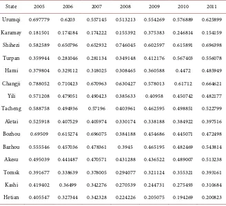
Table A12. Financial intermediation efficiency (FAE).

State 2005 2006 2007 2008 2009 2010 2011

[image:20.595.210.538.415.714.2]

(21)

[image:21.595.208.539.89.370.2]

Table A13. Financial savings structure (FSS).

State 2005 2006 2007 2008 2009 2010 2011 Urumqi 0.422346 0.40234 0.330496 0.367721 0.354564 0.345579 0.360333 Karamay 0.308457 0.340155 0.420742 0.486739 0.270846 0.190032 0.248954 Shihezi 0.714794 0.69827 0.634055 0.66421 0.652411 0.619401 0.634914 Turpan 0.636151 0.598693 0.538841 0.641119 0.623752 0.587966 0.585628 Hami 0.654637 0.606906 0.540217 0.579383 0.578141 0.532667 0.528165 Changji 0.660986 0.647723 0.606712 0.524746 0.568334 0.521205 0.503939 Yili 0.631665 0.598307 0.563083 0.573227 0.544811 0.510391 0.509123 Tacheng 0.665733 0.634592 0.593654 0.616383 0.587476 0.569602 0.567508 Aletai 0.553841 0.483048 0.468487 0.487347 0.473037 0.424532 0.410186 Bozhou 0.563307 0.543743 0.475394 0.500606 0.473282 0.483464 0.471576 Bazhou 0.597043 0.568337 0.554938 0.577428 0.580279 0.567798 0.548597 Akesu 0.614146 0.582832 0.541842 0.575296 0.553754 0.58487 0.535151 Tomsk 0.557732 0.540129 0.484675 0.439257 0.438603 0.408035 0.379598 Kashi 0.585564 0.6638 0.653504 0.688631 0.515092 0.455462 0.453075 Hetian 0.497292 0.502297 0.486045 0.434444 0.406104 0.412961 0.392327

Note: financial savings structure FSS= resident savings/all deposits.

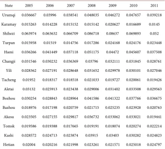
Table A14. The depth of insurance (IND).

Shihezi 0.063974 0.063632 0.066709 0.086718 0.08637 0.069893 0.052 Turpan 0.015958 0.01519 0.014756 0.017286 0.024168 0.024176 0.023448

[image:21.595.209.539.414.711.2]