::::::-··:::::: ... ::·:.:::.::··:·=·
with Genetic Algorithms
"~" ~®
1991 Honours Project: Mark
Botting
-..
.
-..
-..
-.. -..
Optimising Hashing Functions with Genetic Algorithms
Abstract
Genetic algorithms (aka GA's) are a robust global search strategy that ignore
local minima and irrelevant parameters, suitable for large search spaces.
It
is based on
an analogy with natural evolution and survival of the fittest. A generation of potential
solutions is formed by randomly mating pairs from the previous generation, giving
preference to the better performers. By repeating the process many times a (near)
optimal solution evolv~s.
Hashing functions are an implementation for fast table lookup, searching, etc.
Given a symbol to store or lookup in a table, a hashing function produces an index into
the table, preferably such that all possible symbols will be evenly distributed
throughout the table. Their effectiveness is controlled by various parameters such as
table size, symbol distribution, and the f01m of the function itself.
This project aims to couple these two areas together to optimise the parameters
of a given hashing function, by seaching for a good set of values for the parameters
with a genetic algorithm.
Aims and Objectives
The performance of hashing functions are very dependent on their parameters.
So the values of the parameters must be chosen carefully. There are no obvious
methods for choosing the.values. Often the method of choice is a combination of ad hoc
with trial and error.
Choice of a hashing function consists of two things. Choice of an algorithm and
choice of parameters for the algorithm. My project does not aim to cover the first but
rather applying genetic algorithms as an approach to choosing the parameters.
Essential elements consist of software to implement the genetic algorithm,
appropriate codings of the parameters and an evaluation function to measure the
performance of particular parameters. The genetic algorithm has ah-eady been
implemented by GENESIS. The evaluation function should be sufficiently general to
allow different hashing algorithms and parameter codings to be easily 'plugged in'.
My aim is to produce a system for optimising a hashing function. Before
r7
optimisation can be achie~
j§
required a sample of input and the ranges of what
parameters that can be varied.
The file containing the sample data should contain each item on a separate line in
ASCII format. To improve efficiency, it will be read into memory only once.
Obviously larger files will require more processing increasing the run time required for
optimisation. The name of the file is passed to the evaluation function as a GENESIS
application argument.
To evaluate a genotype, the evaluation function is applied to each of the items
from the sample. Statistics are maintained about values produced and the effort required
(for estimating speed). After hashing all items the statistics are combined to form
penalty score which is returned to GENESIS. By changing the ways the statistics are
combined different performance aspects can be emphasised.
Genetic Algorithms
Analogy with Evolution
The concept of genetic algorithms was drawn from the process of natural
evolution. So it will be useful to begin by explaining the similarity. ~ginning
t~-~J!~!wre_was12.i:i~!dial~_ful!o~g !2YAinC?_~a11r; agd tllen
~n~es, before~endinK{!_t!_a step~ckward&1)_wjth hg111J>_S~~ns. How did this happen?
The prooafillity of us evolving randomly is mind bogglingly low! ... Or is it?
The essential element is simply "survival of the fittest". When two organisms
reproduce they combine their structural information (genes) together to form a new but
similar organism. The new combination of genes may gain the child the advantages of
both parents. The child will then be more likely to survive, to reproduce itself and
continue the species with its superior genes. However
if
the child gains the
disadvantages of both parents, it is less likely to survive, and thus the inferior genes are
less likely to continue, effectively removing them from the species.
As time passes the gene pool of the species will become static. The number of
new genetic combinations that are possible will become fewer as superior genes begin
to dominate, and inferior genes are weeded out. Cosmic rays, dietary chemicals, atomic
bombs, etc can cause random mutations within the gene pool, from which novel genetic
combinations can be produced. This occasional genetic stirring thus allows further
evolution of the species.
Overall the average quality of the species improves with each successive
generation. The superior organisms of the population dominating over the inferior.
Over the millenia the population evolves to become better and better at living within
their environment. The population may split to form separately evolving species, each
developing to take advantage of their changing environment in different ways.
Conceptual Model
With ourselves as evidence,
it
is obvious that evolution is a very powerful
strategy for finding organisms ideally suited to their environments. By analysing the
processes that are occurring in evolution, we can construct an algorithm that mimics the
powerful search ability of evolution.
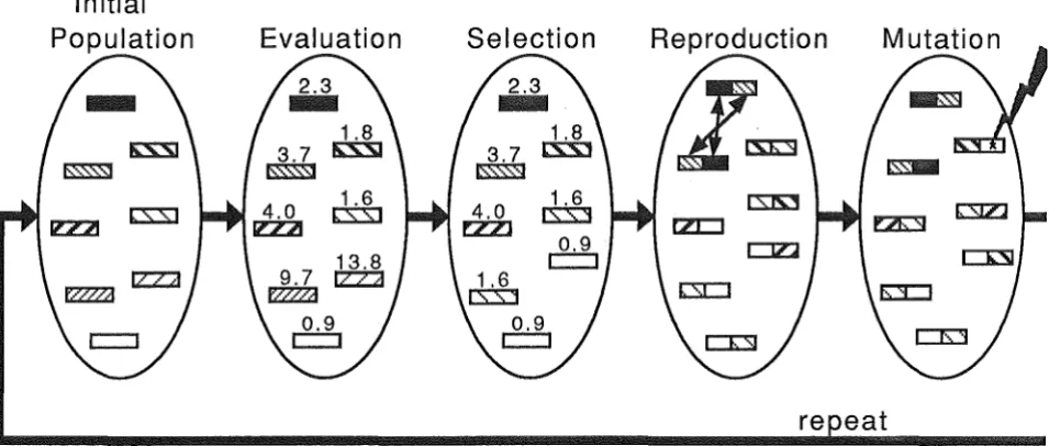
At a simplistic conceptual level, a genetic algorithm consists of the sequence
shown in figure
1.
Initial
Population
Evaluation
Selection
[image:3.597.74.552.437.640.2]re eat
Figure
i.
Simple conceptual model of genetic algorithm.
An initial population is chosen at random. Usually a fixed size of population is
used to simplify details of the algorithm.
In
particular, concerns of population
explosions or extinction can be ignored. Each member, called a structure, of the
population is analogous to an individual organism in evolution.
Optimising Hashing Functions with Genetic Algorithms
with the software I am using, which optimises by minimising the evaluation function,
the performance measure is best thought of as a penalty. Smaller values conferring
better survival.
)\
A new population is created by choosing structures at random from the old
~
z,
~!~
\ ~.
population. Higher probabilities of being chosen are given to the better performers.
<
o-This produces a population in which the superior structures are strongly represented,'
while the number of weaker structures is diminished. This is analogous to survival of
the fittest for natural evolution.
The structures that have survived to the new population then reproduce. Pairs
are chosen at random and mated by swapping portions of information between each
other. The crossover of structures closely represents the exchange of information that
occurs in biology when fertilisation occurs. Some structures gain the benefits of both
parents, some gain the problems of both parents, others find useful new combinations
that consist of otherwise irrelevant parameters.
Finally there is an occasional mutation. As said before this prevents the species
getting in a deadend alleyway with nowhere else to go. Mutations should not happen
too often, which can unnecessarily cause damage to otherwise healthy structures.
Other more complex reproduction operators are available which more closely
mimic the processes of reproduction in biology.
Coding of structures
A structure is best implemented as a binary string, usually of fixed length for
simplicity. Variable length structures are sometimes more appropriate, particularly for
structures which may contain varying amounts of information, but also for special
applications. GENESIS, software which provides most of the functionality of genetic
algorithms that I require, only permits fixed length strings. The binary string is
analogous to the DNA of cells.
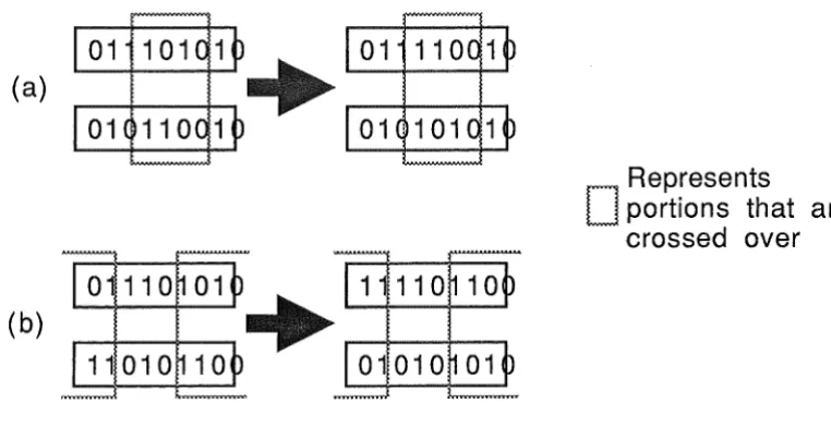
Crossover of pairs of binary strings is easily implemented by simply selecting
two random split points and swapping the bits between them across the two structures.
This treats the string as being circular, the two ends being regarded as joined. Mutation
is also easily implemented as flipping a bit from 1 to
O
or
O
to 1, upon the occurrence of
a random event.
(a)
(b)
1
Represents
D
portions that ar
crossed over
Figure 2. Two examples of crossover.
The internal meaning of the binary string is decoded by the evaluation function,
from which it determines the structures performance. No other part of the genetic
algorithm requires knowledge of the internal coding of the structure. This means that
the design and implementation of the genetic algorithm can be developed independently
[image:4.597.89.470.468.670.2]from the application. For each application, only the evaluation function needs be
written. This feature is exploited by GENESIS to allow the same code to be reused for
any application.
The internal coding is up to the programmer and the particular application, but
usually it consists of a number of numerical parameters gray coded in binary and
concatenated to form a single binary string. Gray coding is very similar to normal
binary except that numbers differ in only one bit position between adjacent values. This
avoids what are termed hamming cliffs.
It is preferable that the combinations possible from the process of crossover are
balanced. For example to go from 128 to 127 requires 8 bit positions to change, but
from 128 to 129 requires only one change. With gray coding only one change needs to
occur to go from 128 to 127 or 129.
decimal
binary
gray
0
0000
0000
1
0001
0001
2
0010
0011
3
0011
0010
4
0100
0110
5
0101
0111
6
0110
0101
7
. 0111 .
0100
8
1000
1100
...
...
. ..
127
0111 1111
0100 0000
128
1000 0000
1100 0000
129
1000 0001
1100 0001
Correspondence of decimal, binary and gray coding of numbers
Hashing Functions
In
general, a hashing function is used to reduce the range of possible values for
its argument to within a smaller range, and to do it quickly. The smaller range is usually
an integer to be used as an index into an array called a hash table. A very common
application is compilers hashing variable names into symbol tables for fast lookup.
The values produced by the hashing function are not necessarily unique for
different argument values. For some applications the function is designed so that
unique values are generated for valid values of the argument. Many software utilities
already exist to generate what are called perfect hashing functions for applications
where the input symbols are known in advance. These software utilities are effective
and efficient, thus this project does not aim to cover them.
A collision occurs when a hashing function produces the same value for two
different arguments. Many techniques exist for resolving the collision which include:
- rehashing. The hash value is repeatedly hashed again until giving a value not
already used.
- separate chaining. The hash table is an array of linked lists.
- linear chaining.
If
the entry in the hash table is already used, then use the next
Optimising Hashing Functions with Genetic Algorithms
Hashing functions should be fast. The primary reason for their use is speed. To
search an array for an item is an O(n) algorithm, or O(log n) if the array is sorted. Hash ·
tables are nearly 0(1) for hash tables with few collisions. This figure degrades as the
number of collisions increases.
The number of collisions can be reduced by ensuring that the distribution of
values produced by the hash function are as close to as uniformly distributed as
possible. This is the major factor in differentiating between a good hashing function
and a bad hashing function. The distribution for a given hashing function may vary for /
··z
different distributions of input items. For example an input that consists of just
i ,
numbers is a different input distribution from just uppercase identifiers.
1
The number of collisions can also be controlled by controlling the utilisation of
the hashtable. When the table reaches some threshold ratio of unused locations to total
table size, the size of the table might be increased to reduce the frequency of collisions.
Likewise if the table empties below some second threshold ratio due to deletions, the
table size may be reduced to reclaim the memory for some other use. This technique
requires that the hashing function will perform well for many table sizes.
For the purposes of this project optimisation will be defined as finding the set of
parameter values for a given hashing algorithm that minimises the time required to hash
an item and resolve collisions; ie the time to obtain the entry
in
the hash table for that
item. Finding a flat distribution is implicit in minimising the time for collision
t.,µic)"'v, ...
resolution.
,
- ~
GENESIS
GENESIS is a complete system for function optimisation using simple genetic
search techniques. This was obtained by ftp and has made my project much simpler.
Originally I expected to have to implement something similar myself.
All that GENESIS requires is a user defined evaluation function which is to be
optimised and the size of the binary strings to be manipulated. Also provided is a utility
that generates code to decode the binary strings into parameters for the evaluation
function, using a description of the number, type, range of the parameters.
The setup command takes a file containing C source code implementing the
evaluation function and compiles it into a program to run the genetic algorithm
experiment. The file also contains comments that allows setup to generate interface code
that decodes a structure and pushes the values onto the stack as parameters to the
evaluation function. Setup also prompts for various arguments and options that control
the operation of the genetic algorithm code.
At the end of the experiment a report of statistics for the experiment is produced
and a dump of the best performing structures. The report is particularly useful for
determining the degree of convergence within the population towards a particular point
of the search space.
See the documentation in appendix A for further details.
Universal hashing algorithm
Originally I had hoped to be able to discover an ideal hashing algorithm for a
given set of conditions by searching the space of possible machine code programs of
some limited length. The binary string of a structure could be interpreted as a sequence
of machine instructions and operands for some pseudo machine. For example a
disassembled routine and the number of bits estimated to code the instruction might be:
rO = O
:labell
rO
<<=
2
rl = [nextchar]
rO += rl
rl
<<=
1
rO += rl
if [morechar] branch :labell
rO %= [tablesize]
8
8+16
8
8+4
8
8+8
8+16
8
However the number of bits required to code this I estimate to be about 108
bits. This particular example is a rather compact routine so the length of the structure
should be say
200
bits. For a structure length of
200
bits GENESIS suggests a
population size of
30000,
and total of
6000000
trials. From practical experience, each
evaluation I would estimate to require at least 2 seconds. Thats a minimum of four and
a half months of CPU time for such an experiment (running on a SparcStation doing 28
MIPS). Thats a long time to wait before discovering any bugs!
Even executing the genetic algorithm with fewer than suggested number of trials
would be beyond my available processing power. So I dropped this approach early in
the year. Instead I am going to concentrate on tuning existing hashing algorithms.
With sufficient resources,
it
would be interesting to try this experiment to
discover what develops.
Optimisation of an . iterative accumulation form
A common application of hashing functions is in compilers to store identifiers
into a symbol table. Many of them can be generalised to the following form.
ho
=o;
hi= hi-1
*
k + Ci
for
1 s i s n;
H(c1c2c3 .. ,en) = hn mod tablesize;
Where the e's are the characters of the identifier being hashed, k is some
constant, and H is the hashing function. The previous form can be further generalised
as the following.
[ (hi-1
a
x)
b
(ci
d
y)]
I
z
for
1 s i s
n;
H(c1c2c3 ... en) = hn mod tablesize;
Where x, y, z are constants and
a,
b, d, I
are operators from the set {-, +, /, *,
&, I,",··}.-,+,/,* are normal integer arithmetic operators.&, I," are the C bitwise
operators 'and', 'or', 'exclusive or' respectively ... is the 'left' operator which
evaluates to its left hand operand. It is included to bring the number of operators up to
eight which can be conveniently represented with three bits.
This generalised form offers seven parameters for optimisation; three integer
values and four operators. These can be coded as a structure for the genetic algorithm
by concatenating the binary (in gray code) representations of each. The integers are
represented with
16
bits each, allowing values in the range Oto
65535
inclusive. The
resulting structure is
60
bits
in
length.
Generally hash tables for compilers will not be larger than
3000.
That means at
most modulo
3000
arithmetic. The operators-,+,*,", .. operating on numbers greater
Optimising Hashing Functions with Genetic Algorithms
not have equivalences but are not such important operators. Also I feel 65535 should be
a large enough range to give the operators a chance to be useful.
32 bits would have been just as useful as (if not better than) 16 bits except that
the number of trials needed for convergence increases exponentially with the length of
the structure. Trading off against that was the observation that larger values for the
parameters seemed to give better performers in general. Many present day CPUs are
capable of 16 arithmetic, thus the results are reasonably portable.
Measurement of hashing time
_Empirical measurements_are better than theozy..whenitc..001_estUJh~~I~~Lw2rld.
However empirical measurement of speed is not practical where the operations of the- ,
hashing function can be optimised for certain values and operations. The obvious
example is multiplication by powers of two, which can be optimised as left shifts. The
optimisations cannot be performed at compile time as the parameters and operators are
not known at that time. Optimisation must occur at runtime for each evaluation of a
structure.
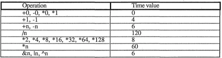
To obtain an estimate of the time involved in hashing, a runtime analysis of the
operations and their operands must be made. When an operation is interpreted, a
number of time units representative of the speed of the operation are added to the total
time so far for the evaluation. Operations that may be optimised for special operands
add a modified time factor. The timings and optimisations that are being used are:
Operation
Time value
+O, -0, *O, * 1
0
+l, -1
4
+n, -n
6
In
120
*2, *4, *8, *16, *32, *64, *128
8
*n
60
&n, In, An
6
Measurement of collision resolution time
In
measuring the distribution of values produced I have assumed the use of
separate chaining to resolve hashing collisions. In most cases extending it for other
collision resolution methods simply requires implementing the collision resolution part
of the hashing function.
Separate chaining maintains a linked list for each hash location of all items that
hash to it. To find an item in the hash table involves hashing it to find its hash location
and then scanning the linked list at that location. So the time for collision resolution is
the time used to scan the linked list the particular hash location. The average length of a
linked list is dependent upon the distribution of hash values produced by the function .
... ®
.. ..
•
-.. -..
-Figure 3. Form of hash table.
'2_ (
[image:8.597.66.488.341.452.2]The empirical approach to determining the collision resolution time has a
number of advantages. It easily allows different distributions of items to hash by
specifying a file of sample input. Methods of implementation are obvious.
Im~ementing_a theQretic;al clllalysis seems to_b~ i!!m!actical
at1c:l
non-trjyifil. It is easily
?.
acfapledror other hashing algorithms. The only major disadvantage is the long
·
execution time involved.
The method is to hash each of the items read from a representative sample file as
if hashing for a specific application. A total of the time used is accumulated as each item
is hashed. A table is maintained of the length of the linked list for each hash location.
After all the items have been hashed, the pe1formance penalty is the average time to
hash each item.
1
In the early stages of evaluation function development ~aiious statistical
methods were used to determine the actual distribution of hash locations used. This
allowed me to see how effective my evaluation scheme was. Each statistical method
produced slightly different results, in particular most methods were dependent on the
hash table size. Varying the size of the table generally gave larger tables a worse
measure of distribution, even though the same number of identifiers have been hashed
to the same shaped distribution. Another (possibly related) effect was the size of the
hash table compared to the number of sample items hashed. Variance of the number of
hashes to each location seemed to give the best results when the table size was fixed.
The statistical calculation below seemed to give a measure of distribution
independent of table size, but did not give as good results as variance when the table
size was fixed.
sumdiff
:=
O;
foreach index i
sumdiff := sumdiff
+
abs(mean -
freq[i]);
flatdistribution
:=
sqr(sumdiff)/tablesize;
Calculating the flat distribution.
Resu Its
After a run of 240000 evaluations on a population of 2000 structures with a
fixed table size of 1403 the best structure decoded as:
[ (hi-1 -
26096) /\
(Ci
k1)]
k2
where kl and k2 are some constants that have no effect due to the .. operator.
Hence it can be simplified to:
·
(hi-1 -
26096) /\
Ci
The fact that the operators/,
&
and
I
aren't very useful is not surprising when
some consideration is given to their effect on their operands. Integer division evaluates
to a disproportionately large number of zeroes. Bitwise and tends to produce values that
contain lots of zero bits. Similarly bitwise or tends to produce values with lots of one
bits. All three operators share the property of discarding information without using it.
The other operators reduce the amount of information but not without using it for some
effect on the end result.
Subtraction and addition of a constant value are equivalent in modulo arithmetic.
It is merely chance that the genetic algorithm chose one over the other.
Optimising Hashing Functions with Genetic Algorithms
Conclusion
Genetic algorithms are a very powerful search strategy. Although powerful, for
particular applications there may be more efficient strategies already available. They are ./
well suited to optimising the parameters of hashing functions, especially as the is no
"'
other obvious strategy, except for exhaustive search.
Exhaustive search is not really an option. To try every 60 bit value would
require 260
>
1Q18
evaluations. At an optimistic 10 evaluations per second, thats longer
than 3 billion years. A simple genetic algorithm might require 500000 trials for a
largeish experiment which is about five days at a slow one evaluation per second. Five
days is a long time, but for a one off experiment it is acceptable.
. With 1;1ore time I could have made comparisons between various different /
I
hashmg algonthms.
·
e
As an aside. The idea of using genetic algorithms to develop small programs
using the approach given under the heading of 'Universal hashing algorithm' is worthy
of further research. Variable length stmctures coupled with appropriate reproduction
operators could be used to make the search more efficient.
References
David
E.
Goldberg. "Genetic Algorithms in Search, Optimization & Machine
Learning". Addisson-Wesley, 1989. ISBN 0-201-15767-5.
B.J. McKenzie,
R.
Harries, T. Bell. "Selecting a Hashing Algorithm",
Software-Practice and Experience, Vol. 20(2), pp 209-224, (Feb 1990).
John H. Holland. "Adaption in Natural and Artificial Systems". University of
Michigan Press, 1975. ISBN 0-472-08460-7.
'·,":,._!5.:jluth. "The Art of Computer Programming".
, ·
John F. Grefenstette. "User's Guide to GENESIS 1.2ucsd". Documentation
available with GENESIS.
"GENESIS". Source available via anonymous ftp from the Artificial Life
archive server, iuvax.cs.indiana.edu (129.79.254.192) in the
pub/alife/software/uni:x/GAucsd directory.
Appendix A - GENESIS documentation
Oct 4 15:15 1991 root:/tmp/3607.lwf_tmp Page 1
A User's Guide to GENESIS 1.2ucsd
written by John J. Grefenstette
Navy Center for Applied Research in Artificial Intelligence Naval Research Laboratory
Washington, D.C. 20375-5000
modified by Nicol N. Schraudolph
Computer Science & Engineering Department University of California, San Diego
La Jolla, CA 92093-0114
ABSTRACT
This document describes the GENESIS system
for function optimization based on genetic search
techniques. Genetic algorithms appear to hold a
lot of promise as general purpose adaptive search
procedures. However, the authors disclaim any
warranties of fitness for a particular problem.
The purpose of making this system available is to
encourage the experimental use of genetic
algo-rithms on realistic optimization problems, and
thereby to identify the strengths and weaknesses
of genetic algorithms.
August 14, 1987
Note:
GENESIS 1.2ucsd was derived from GENESIS 4.5
by Nicol Schraudolph at UCSD. It is available via
anonymous ftp from the Artificial Life archive
server, iuvax.cs.indiana.edu (129.79.254.192) in
the pub/alife/software/unix/GAucsd directory. Bug
reports and comments on this version should be
di-rected to nici%[email protected]. GENESIS 4.5 may be
obtained from its author at [email protected].
November 14, 1990
A User's Guide to GENESIS 1.lucsd
written by John J. Grefenstette
Navy Center for Applied Research in Artificial Intelligence Naval Research Laboratory
Washington, D.C. 20375-5000
modified by Nicol N. Schraudolph
Computer Science & Engineering Department
University of California, San Diego La Jolla, CA 92093-0114
l·
IntroductionThis document describes the GENEtic Search
Implementa-tion System GENESIS l.2ucsd. The system was written to
promote the study of genetic algorithms for function
minimi-zation. GENESIS runs under the UNIXt operating system,
ver-sion V7 or higher. Since genetic algorithms are task
independent optimizers, the user must provide only an
"evaluation" function which returns a value when given a
particular point in the search space. The system is written
in the language c. Details concerning the interface between
the user-written function and GENESIS are explained below. Shell files are provided to ease the construction of genetic algorithms for the user's application.
This section provides a general overview of genetic
algorithms (GA's). For more detailed discussions, see
[518]. GA's are iterative procedures which maintain a
"population" of candidate solutions to the objective
func-tion f(x):
P(t) = <xl(t), x2(t), ••• , xN(t}>
Each structure xi in population Pis simply a binary
string of length L. Generally, each xi represents a vector
of parameters to the function f(x), but the semantics
asso-ciated with the vector is unknown to the GA. During each
iteration step, called a "generation", the current
popula-tion is evaluated, and, on the basis of that evaluapopula-tion, a
new population of candidate solutions is formed. A general
sketch of the procedure appears in Figure 1.
t UNIX is a trademark of Bell Laboratories.
- 2
-t <- O;
initialize P(t); -- P(t} is the population at time t evaluate P (t);
while (termination condition not satisfied) do begin
t <- t+l;
end;
evaluate P{t);
Figure 1. A Genetic Algorithm
The initial population P(O) is usually chosen at
ran-dom. Alternately, the initial population may contain
heu-ristically chosen initial points. In either case, the
ini-tial population should contain a wide variety of structures.
Each structure in P{O) is then evaluated. For example, if
we are trying to minimize a function f, evaluation might
consist of computing and storing f{xl), ••• , f{xN).
The structures of the population P{t+l) are chosen from
the population P(t) by a randomized "selection procedure"
that ensures that the expected number of times an structure
is chosen is proportional to that structure's performance,
relative to the rest of the population. That is, if xj has
twice the average performance of all the structures in P(t),
then xj is expected to appear twice in population P(t+l).
At the end of the selection procedure, population P{t+l)
contains exact duplicates of the selected structures in
population P{t).
In order to search other points in the search space,
some variation is introduced into the new population by
means of idealized "genetic recombination operators." The
most important recombination operator is called "crossover".
Under the crossover operator, two structures in the new
population exchange portions of their binary representation.
This can be implemented by choosing a point at random,
called the crossover point, and exchanging the segments to the right of this point. For example, let
xl
=
100:01010, andx2 = 010:10100.
and suppose that the crossover point has been chosen as
indicated. The resulting structures would be
yl
y2
100:10100
010:01010.
- 3
-and
Crossover serves two complementary search functions. First,
it provides new points for further testing within the
sche-mata already present in the population. In the above
exam-ple, both xl and yl are representatives of the schema
100#####, where the# means "don't care". Thus, by
evaluat-ing yl, the GA gathers further information about this
schema. Second, crossover introduces representatives of new
schemata into the population. In the above example, y2 is a
representative of the schema #1001###, which is not
represented by either "parent". If this schema represents a
high-performance area of the search space, the evaluation of
y2 will lead to further exploration in this part of the
search space.
evaluations, or some other application dependent criterion.
The basic concepts of GA's were developed by Holland
1975 (8] and his students [2,4,7,9]. Theoretical
considera-tions concerning the allocation of trials to schemata [4,8]
show that genetic techniques provide a near-optimal
heuris-tic for information gathering in complex search spaces. A
number of experimental studies [2,3,4] have shown that GA's
exhibit impressive efficiency in practice. While classical
gradient search techniques are more efficient for problems
which satisfy tight constraints {e.g., continuity,
low-dimensionality, unimodality, etc.), GA's consistently
out-perform both gradient techniques and various forms of random search on more difficult {and more common) problems, such as
optimizations involving discontinuous, noisy,
high-dimensional, and multimodal objective functions. GA's have
been applied to various domains, including numerical
func-tion.optimization [2,3], adaptive control system design [5], and artificial intelligence task domains [11]. The next sec-tion discusses each of the major modules of this implementa-tion in greater detail.
l·
Major ProceduresInitialization
File "init.c" contains the initialization procedure,
whose primary responsibility is to set up the initial
population. If you wish to "seed" the initial population
with heuristically chosen structures, put the structures in
the "init" file {see "Files") and use the ' i ' option (see
"Options"). The rest of the initial population is filled
with random structures, or by a reduced-variance technique for super-uniform initialization if the 'u' option is used.
- 4
-Generation
As previously mentioned, one generation (see
"generate. c") comprises the following steps: selection,
mutation, crossover, evaluation, and some data collection
procedures.
Selection
Selection is the process of choosing structures for the
next generation from the structures in the current
genera-tion. The selection procedure (see file "select.c") is a
stochastic procedure that guarantees that the number of
offspring of any structure is bounded by the floor and the
ceiling of the (real-valued) expected number of offspring.
This procedure is based on an algorithm by James Baker. The
idea is to allocate to each structure a portion of a
spin-ning wheel proportional to the structure's relative fitness. A single spin of the wheel assigns the number of offspring
to all structures. This algorithm is compared to other
se-lection methods in [1]. The selection pointers are then
randomly shuffled, and the selected structures are copied
Oct 4 15:15 1991 root:/tmp/3607.lwf_tmp Page 3
After the new population has been selected, mutation is
applied to each structure in the new population. (See
"mutate.c".) Each position is given a chance (=M rate) of
undergoing mutation. This is implemented by computing an
interarrival interval between mutations, assuming a mutation
rate of M rate. The MUTATION macro in "define.h"
deter-mines what happens if mutation does occur; the default ac-tion is to flip the bit value for that posiac-tion. The mutated structure is then marked for evaluation.
Crossover
Crossover (see "cross.c") exchanges alleles among adja-cent pairs of (C rate*Popsize) structures in the new
popula-tion. Note that-a Crate greater than 1.0 will cause some
structures to undergo several crossovers. Crossover might be implemeneted in a variety of ways, but there are theoretical advantages treating the structures as rings, choosing two crossover points, and exchanging the sections between these
points [4]. The segments between the crossover points are
exchanged, provided that the parents differ somewhere
outside of the crossed segment. If, after crossover, the
offspring are different from the parents, then the offspring
replace the parents, and are marked for evaluation. In the
"setup" program Crate is entered interms of the expected
number of crossing points per bit, a measure that directly
indicates the disruptiveness of the crossover procedure.
- 5
-3. Evaluation Procedure
To use GENESIS, the user must write an evaluation
pro-cedure. There are three levels of abstraction at which such
a procedure may be written. At the lowest level a function
called "eval" receives a pointer to the genome and its
length in-bit as input and returns a double precision value. It must be declared as follows:
double eval(genome, length)
char genome[]; int length;
The interpretation of the genome is entirely up to the user, thus allowing great flexibility and efficiency. However, the packed form of the genotype can be awkward to deal with if
the parameters are not aligned with byte boundaries.
There-fore an evaluation function "eval" may be declared instead
which receives an unpacked genotype:
double eval(buff, length) char buff [];
int length;
where buff is a character array containing (integer) O's and l's, and length indicates the length of the array buff. This form of evaluation function was used in the original GENESIS and is assisted by some functions which facilitate the
in-terpretation. One is called Ctoi:
double Ctoi(buf, length) char buf[];
int length;
which takes two arguments, a pointer to a char array and a
length indicator. Ctoi() returns the value computed by
in-terpreting the buffer as an unsigned binary string with the
indicated length. If the 'A' option is used, Ctoi() will
add a random fractional part to the value in order to avoid aliassing effects that might otherwise compromise the search of continuous spaces (see "Options").
Gray codes are often used to represent integers in
ge-netic algorithms. They have the property that adjacent
in-teger values differ at exactly one bit position; their use
avoids the unfortunate effects of "Hamming cliffs" in which adjacent values, say 31 and 32, differ in every position of
their fixed point binary representations (01111 and 10000,
respectively). Functions which translate between Gray code
and fixed point representations are provided:
Gray(inbuf, outbuf, length) char *inbuf, *outbuf; register int length;
Degray(inbuf, outbuf, length) char *inbuf, *outbuf; register int length;
.6
-In the function Gray, "inbuf" contains the fixed point
integer, one bit per char. "outbuf" gets the Gray coded
version, one bit per char. In Degray, "inbuf" contains the
Gray code integer, one bit per char; "outbuf" gets the
corresponding fixed point integer.
A procedure Error() is provided which writes an error message to the file "log.error" and to stderr, and then
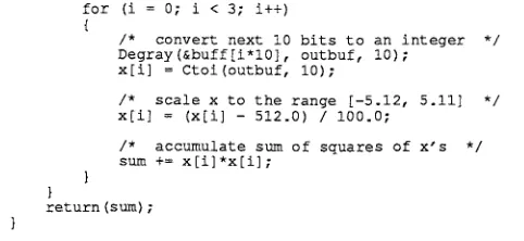
t'.er-minates the program. Figure 2 shows an evaluation procedure
which uses these GENESIS procedures. Note how a call to the
evaluation function with negative "length" parameter is used
!****************************************** file fl.c ****/
double eval(genome, length)
char genome[]; int length;
{
register int i; char buff[30]; char outbuf[lO]; double sum= 0.0;
/* phenotype description, must be static*/ static double x[3];
/* return previous phenotype on request */
i f (length < 0)
sprintf(genome, "\n%lf %lf %lf", x[O], x[l], x[2]); else
·{
/* Galength 30 */
if (length != 30) Error("length error in eval");
I
{
I* convert next 10 bits to an integer */
Degray(&buff[i*lO], outbuf, 10); x[i] = Ctoi(outbuf, 10);
I* scale x to the range [-5.12, 5.11] */
x[i] = (x[i] - 512.0) I 100.0;
I* accumulate sum of squares of x's */
sum+= x[i]*x[i];
return (sum};
******************************************* end of file****/
Figure 2: An Evaluation Function.
7
-by GENESIS to ask for a phenotypic description of the most
recently evaluated individual. This description is provided
automatically if you use the "wrapper" (see below) and will
be printed in the "min" file.
It is often desirable to pass parameters to the
evalua-tion function that might vary from experiment to experiment
but should not be subjected to the GA search. GENESIS uses
a method similar to that of passing C command line arguments to make such "application-specific" parameters, entered via the "setup" program, accessible through the declarations:
extern int GArgc;
extern char *GArgv[];
which the wrapper (see below} provides for you. Note that
each of the GArgc string parameters in Gargv[] may contain
blank spaces but not '\0' or '\n'.
The Wrapper
This version of GENESIS includes an awk(l} script
called "wrapper" which provides a higher level of
abstrac-tion: i t allows the direct use of most c functions as
eva-luation functions. The only restrictions are:
- the function must not be called "_ eval";
- i t must return a scalar type or a pointer to such a type;
- all its parameters must be simple C types as described
below, or pointers to such types (this allows for passing arrays by reference).
The wrapper gets invoked from the "setup" program and
constructs from a file <name>.c the file <name>-ga.c which
includes a function" eval(gene, length)" which interfaces
/* GAeval <fn> <fieldl> <field2> ••• *I
where <fn> is the name of your fitness function, possibly
prefixed with an asterisk for indirect return values. It
is followed by one or more fields, where each field
speci-fies a parameter to the fitness function. White space
de-limits fields and hence may not occur within fields. The
format of an individual field is (in this order):
1) an integer indicating the number of bits to be used for
representing this parameter on the genotype. This must
be between 1 and the number of bits of an "int" on your machine to make sense.
- 8
-2) (optional} a colon followed by a number r specifying the
range of the parameter. This means that the parameter
will range from -r (or zero if unsigned - see below}
in-clusive to +r exin-clusive. If omitted, the range is deter-mined directly from the number of bits used to represent
the parameter. A second numbers, separated by a colon,
may be specified, forcing a range from r inclusive to s
exclusive. Both rands may contain a decimal point and
a sign, but no exponent, ands must be strictly greater
than r.
3) a character string containing in any order, in upper or lower case:
4)
a} exactly one of 'c', 's', 'i', 'l', 'f' or 'd',
specifying the parameter type as char, short, int, long, float or double respectively;
b} (optional} a 'b' or 'g' indicating that the parameter is to be encoded in binary or Gray code, respectively.
Either character causes the parameter to be left alone
by the DPE algorithm (see below} which relies on the de-fault Gray coding for its operation.
c) (optional) a 'u' indicating that the parameter is
un-signed. For float or double parameters the type will
not change, but the default range will be from zero t o r instead of -r t o r (see above).
(optional} an integer n indicating replication: the
parameter is a pointer to an array of n values of the
format given in 1) - 3). Values of 1 (simple
indirec-tion) or O (same as non at all} for n are allowed.
Space for parameters on the genotype is allocated from the
left in order of the fields. The following figure
demon-strates how the evaluation function of Figure 2 is greatly simplified when the wrapper is used:
/**************************************** file fl.c ****/
double f l (x)
register double *x;
[image:15.843.57.298.69.180.2]Oct 4 15:15 1991 root:/trnp/3607.lwf_trnp Page 5
/* accumulate sum of squares of x's *I
for (sum= 0.0, i = O; i < 3; i++) sum+= x[i]*x[i];
return (sum);
I* GAeval fl 10:5.12d3 */
/**************************************** end of file****/
Figure 3: Sarne Evaluation Function using the Wrapper.
- 9
-!·
Dynamic Parameter EncodingWhen encoding real-valued parameters of the evaluation
function on a binary genotype there is a conflict between
the desire to keep the genes short for fast convergence and
the need to know the result with a certain precision. An
appropriate - but cumbersome - reaction when faced with this dilemma would be to first run a simulation with short genes to quickly obtain a low-precision result, then repeating it with ever-increasing precision while keeping the genotype short by restricting the search to the previously identified solution region.
Dynamic Parameter Encoding (DPE} [10] implements this stra-tegy of iterative refinement by gathering convergence
sta-stistics of the top two bits of each parameter. Whenever
the population is found to be converged on one of three
sub-regions of the search interval for a parameter, DPE invokes
a "zoom" operator that alters the interpretation of the gene in question such that the search proceeds with doubled
pre-cision, but restricted to the target subinterval. In order
to minimize its disruptiveness the zoom operator preserves most of the phenotype population by modifying the genotypes to match the new interpretation.
The DPE algorithm logs its zoom activity in the "dpe" file (see "Files"). Since the zoom operation is irreversible it has to be applied conservatively in order to avoid premature
convergence; to this end DPE srnoothes its convergence
sta-tistics through exponential historic averaging. The time
constant of this filtering process is an important
characte-ristic of the algorithm: the smaller its value, the bolder
DPE becomes, accenting the risks and benefits associated
with fast convergence.
Note that although DPE often facilitates a radical reduction
of gene length, there is a point beyond which the function
to be optimized will no longer be sampled with enough
reso-lution to yield useful results. In particular if the basin
of attraction around the optimum is small, a low-resolution
search might miss it altogether. Of the five test functions
included with GENESIS for instance, four can be solved with
DPE using as little as three bits per parameter, but the
rnultirnodal function f5 requires twice as much.
The DPE algorithm is activated by selecting a non-zero smoo-thing time constant in the "setup" program; it may be selec-tively disabled for certain parameters via a 'b' or 'g' flag in the GAeval comment line (see "Wrapper"). Since DPE is based on strong assumptions about the interpretation of the genome it is meant to be used in conjunction with a C-style
evaluation function as facilitated by the wrapper.
This quick overview was intended to encourage and facilitate first experiments with the DPE algorithm; many aspects have
been somewhat glossed over. For a more detailed description
and discussion of the DPE algorithm and its correct applica-tion please refer to [10].
10
-5. Installing the System
Some system tailoring may be necessary when installing
GENESIS on a new machine. All of these changes are in the
GENESIS source directory.
1) If you can't receive mail on the local host, modify the mail address in file "ex" accordingly, or remove the mail command altogether.
2) Check the top section of file "define.h" - i f you are on a non~standard UNIX system, you may have to modify it. 3) If awk(l) is not available on your system, you will not be able to use the wrapper or the "ex" command. To use DPE without the wrapper, you will have to define the global
va-riables GAgenes, GAposn, GAbase and GAfact in your
evalua-tion file, which must end in "-ga.c". Please refer to the sample wrapper output file "fl-ga.c" for further details. 4) To compile the system, use the rnake(l) command:
% make all
This should compile the programs and create the library
"ga.a". This library may then be linked to user-written evaluation procedures as shown below.
~- Setting~ Experiments
GENESIS may be set up to run in any directory as follows: 1) Copy the Makefile into the current directory:
% cp GEN/UserMakefile Makefile
where GEN is replaced by the full path name to the GENESIS source directory on your system.
2) To get the other essential files into the current direc-tory, use the command:
% make ga-install
3) run "setup", which prompts for the following (a <er> response to any prompt gets the default in brackets; a'*' indicates that the default is narnically from previously entered data)
the name of the evaluation file [fl]:
parameters: value shown derived
dy-At this point rnake(l) is called to preprocess, compile and
11
--- the suffix for file names [*]:
The filename extension for this experiment (see "Files"); it defaults to the name of the evaluation file. If an "in" file with the chosen suffix exists already, it will be read at this point to be used as default for subsequent prompts. If the existing "in" file is read-only, you will be asked to provide an alternate suffix for writing - thus "setup" may be used to re-edit existing "in" files, or to make modified
copies from a read-only master file. If there is no
appro-priate "in" file, "setup" will create it and try to guess reasonable defaults, with more or less success.
the number of experiments [l]:
(number of independent optimizations of same function) the length of the structures in bits [*]:
If there is a comment of the form"/* GAlength <n> */" - as produced automatically by the wrapper - in the evaluation file, the length suggested will be <n>.
the population size [*):
the number of trials per experiment [*]: the rate of crossing points per bit [*): the mutation rate [*):
the generation gap [1.0]:
The generation gap is the percentage of the population which
is replaced in each generation. Note that GENESIS operates
very inefficiently for small generation gaps. -- the scaling window [-1]:
When minimizing a numerical function with a GA, it is common to define the performance value u(x) of a structure x as
u(x)
=
F - f(x}, where Fis a large baseline function value.Negative values of u(x) can either be zeroed or avoided al-together by setting F to f max, the maximum value that f(x)
can assume in the given-search space. Often f max is not
available a priori, in which case we may use F ~ f(x max),
the maximum value of any structure evaluated so far.
-Either choice of F has the unfortunate effect of making good
values of x hard to distinguish. For example, suppose f max
= 100. After several generations, the current population
might contain only structures x for which 5 < f(x) < 10. At
this point no structure in the population has a performance
which deviates much from the average. This reduces
these-lection pressure towards better structures, and the search
stagnates. One solution is to update the baseline to, say,
F = 15, and rate each structure against this new standard.
The scaling window Wallows the user to control how often
the baseline performance is updated. If W > O, the system
sets F to the greatest value of f(x) which has occurred in
the last W generations. A value of W = 0 indicates an
infi-nite window, ie. F = f(x_max). This window scaling method is
gle "lethal" genotype can all but eliminate selective
pres-sure for W generations. A more robust method studied by
Forrest [6], which we call "Sigma Scaling", is now available with GENESIS, and can be accessed by setting W < 0.
-- the sigma scaling factor [2.0]:
In sigma scaling, Fis set to the average population fitness plus a certain multiple, the sigma scaling factors, of the standard deviation of population fitness. (Individuals worse
than Fare assigned zero performance.) Note that for an
in-dividual x with f(x) one standard deviation better than the
population average, u(x)
=
(s + 1)/s; sigma scaling thusprovides very direct control over the selection pressure. Values for s between 1 and 5 have been used in practice.
-- the smoothing time constant for DPE [OJ:
This is the time constant (in generations} with which the
DPE algorithm smoothes its convergence statistics through
exponential historic averaging in order to avoid premature
convergence. A value of zero switches DPE off altogether.
-- the convergence threshold [*):
The percentage of the population that needs to have the same value in a given allele for it to be considered "converged". Since it is used as the trigger threshold for the zoom
ope-rator, this is an important parameter for DPE. The default
value suggested by "setup" follows an analysis in [10). how many alleles must converge to end the experiment [*]:
(0 indicates that no such check will occur)
how large the bias must be to end the experiment [0.99]: how many consecutive generations without any evaluations occurring will end the experiment [2):
(0 indicates that no such check will occur)
If one of the above three termination conditions is met, the remainder of the experiment will be faked by reprinting the current statistics an appropriate number of times.
the number of trials between data collections [*]: (0 indicates collect at start and end of experiment only) how many of the best structures should be saved [*): the number of generations between dumps [*]:
(0 indicates no dumps will occur)
the number of dumps that should be saved [1]: (0 indicates no dumps will occur)
the options (see chapter 7) [eel]:
the seed for the random number generator [*]:
At this point setup writes all settings out to the "in" file and prompts for application-specific arguments (see chapter
3). Hitting return will get you the default read previously
from the "in" file, or exit the loop when no default exists.
-Oct 4 15:15 1991 root:/tmp/3607.lwf_tmp Page 7
Files
For any the file names listed below, you may create a
direc-tory in which these files are collected. The report for an
experiment with filename extension 11foo", for instance, will
be in the file "foo" in the directory "report" if it exists, in the file "report. foo" in the current directory otherwise. In either case the "clean" command removes all files with a
given extension. There is also a file "log.error" in which
GENESIS error messages are collected.
"ckpt" - a checkpoint file containing a snapshot of
impor-tant variables, and the current population. This file is
produced if the 'd' option is set, the second termination
signal is received, or both the number of saved dumps and
the dump interval are positive. This file is necessary for
the restart option ' r ' to work, but can also be interesting in its own right.
"dpe" - this file, produced when the DPE algorithm is used,
logs the activity of the zoom operator. For each zoom one
line is appended, containing generation and trial number,
the index of the zoomed parameter (starting at zero}, the
endpoints of its new search interval, and its new precision.
"in" - contains all input parameters. This file is required.
"init" - contains structures which will be included in the
initial population. This is useful if you have heuristics
for selecting plausible starting structures. This file is
read iff the option ' i ' is set.
"log" - logs the dates of starts and restarts. This file is
produced if the ' l ' option is set.
"min" - contains the best structures found by the GA. The
number of elements in "min" is indicated by the response to
the "save how many" prompt during setup. If the number of
experiments is greater than one, the best structures are
stored in "min.n" during experiment number n. This file is
produced if the number of saved structures is positive.
"out"- contains data describing the performance of the GA.
This file is produced if option 'c' is set.
"report" - produced by the report program from the "out"
file, this file summarizes the performance of the GA.
"schema" - logs a history of a single schema. This file is
required for the 's' option.
14
-7. Options
GENESIS allows a number of options which control the
kinds of output produced, as well as certain strategies
employed during the search. Each option is associated. with
a single character. The options are indicated by responding
to the "options" prompt with a string containing the
appropriate characters. If no options are desired, respond
'a': evaluate all structures in each generation. This
may be useful when evaluating a noisy function, since it
allows the GA to sample a given structure several times. If
this option is not selected then structures which are ident-ical to parents are not evaluated.
its that due this
'A': causes Ctoi() to add a random fractional part to
conversion results in order to avoid aliassing problems might otherwise occur when searching continuous spaces,
to the quantized nature of the genetic encoding. Since
option makes Ctoi(} stochastic, 'A' always implies 'a'.
'b': at the end of the experiments, write the average best value (over all experiments) to the standard output.
'c': collect statistics concerning the convergence of
the algorithm. These statistics are written to the "out"
file, after every "report interval" trials. The intervals
are approximate, since statistics are collected only at the
end of a generation. Option 'c' implies 'C' but is
computa-tionally more expensive.
·, C' : collect statistics concerning the performance of
the algorithm. These statistics are written to the "out"
file, after every "report interval" trials. The intervals
are approximate, since statistics are collected only at the end of a generation.
'd': dump the current population to "ckpt" file AFTER
EACH EVALUATION. WARNING: This may considerably slow down
the program. This may be useful when each evaluation
represents a significant amount of computation.
'e': use the "elitist" selection strategy. The elitist
strategy stipulates that the best performing structure
always survives intact from one generation to the next. In
the absence of this strategy, it is possible that the best
structure disappears, thanks to crossover or mutation.
' i ' : read structures into the initial population. The
initial population will be read from the "init" file. If
the file contains fewer structures than the population
needs, the remaining structures will be initialized
ran-domly, or super-uniformly if the 'u' option is used.
15
-' l -' : log activity (starts and restarts} in the "log"
file. Some error messages also end up in the "log" file.
'L': dump the last generation to the "ckpt" file. This
allows the user to restart the experiment at a later time,
using option 'r'.
'o': at the end of the experiments, write the average
online performance measure to the standard output. Online
performance is the average of all evaluations during the
experiment.
'O': at the end of the experiments, write the average
Offline performance measure to the standard output. Offline
Oct 4 15:15 1991 root:/tmp/3607.lwf_tmp Page 8
this case, the "ckpt" file is read back in, and the GA takes up where i t left off.
' s ' : trace the history of one schema. This options
requires that a file named "schema" exist in which the first line contains a string which has the length of one structure
and which contains only the characters '0', '1', and'#'
{and no blanks). The system will append one line to the
schema file after each generation describing the performance
characteristics of the indicated schema {number of
representatives, relative fitness, etc.}.
' t ' : trace each major function call - FOR DEBUGGING.
Tracing statements are written to the standard output.
'u': create a super-uniform initial population in which all schemata up to a certain defining length {limited by the
population size} are equally represented. In
crossover-do-minated GAs {with low mutation rate} this eliminates the
risk of pathological initial populations in which an
impor-tant low-order schema just happens to be missing, and has to
be created by an unlikely mutation event. The 'u' option
uses a reduced-variance stochastic algorithm which produces
a population with no local, but large global correlations.
Crossover is very effective in destroying such long-range
correlations, but this option should not be used in
muta-tion-dominated GAs, where crossover rates are too low.
- 16
-~- Running the Programs
A GENESIS program with, say, evaluation file name "fl"
and file name extension "foo" may be started directly by
ty-ping "ga.fl foe". In most cases, however, i t is preferable
to use the "go" or "ex•• shell scripts instead {see below}.
You can terminate a GENESIS program prematurely by sending
it "TERM" signals using the kill{l} command. The first such
signal causes the program to exit after the current
experi-ment is completed; the second forces a "ckpt" dump and imme-diate termination.
The command "go ga.fl foe&" will run the same program
at low priority in the background and then ca.11 the "report" program if appropriate {see below}. "go" can also be used to execute a GENESIS program remotely provided you have the ne-cessary permissions on the remote machine: the command
go ga.fl foe neuromancer gref /data/genesis &
for instance will recompile 11fl.c11 on host "neuromancer" in
the directory "/data/genesis", which must contain a
correct-ly installed UserMakefile. It will then copy "in.foe" (also
"init. foe" and "schema. foo" if applicable} into the remote
directory, run the program there {using login name "gref"},
then copy any resulting data files back into your local di-rectory and produce a report i f appropriate.
to it as directory argument: 11go11 exploits this special case
to avoid the overhead of copying files between the hosts.
If you have GENESIS experiments queued in files you can
execute selected queues by typing ''ex <file name (s} >". "ex"
notifies you via write(l} or mail{l} when all experiments
are completed. "ex" distributes experiments to remote hosts
specified in a file "GAhosts" in either the local directory,
your home directory or the GENESIS source directory, then
runs the remaining experiments (if any} locally. Each entry
in the GAhosts file consists of a load factor {how many pro-grams will be sent to that host} followed by the remote exe-cution arguments to "go" as described above - see the sample GAhosts file in the GENESIS source directory for details.
The Report
If the 'c' or 'C' option is selected, a report
describ-ing the performance of the GA can be produced by the
"report" program, which summarizes the mean and variance of
several measurements, including online performance, offline performance, the average performance of the current
popula 17 popula
-tion, and the current best value. Online performance is the
mean of all evaluations; offline performance is the mean of
all current best evaluations; see [5].
If option 'c' is selected, three additional measures are
printed: "Conv" is the number of positions which have
con-verged at least to the chosen threshold, "Lost" is the num-ber of those which have converged 100% {ie. the entire popu-lation has the same value}, and "Bias" indicates the average percentage of the most prominent value in each position. For instance, a bias of 0.75 means that on average each position has converged to either 75% O's or 75% l's.
9. Example
Figure 3 shows an example of a user-defined evaluation function for the following problem:
Min f (x} sum [ (xi}A2], where -5.12 <=xi<= 5.11, i=l,2,3.
Each xi is represented by 10 bits, so that the structure
length is 30, and the precision for each xi is 0.01. The
minimum occurs at the origin. (Of course, this problem does
not require the full power of genetic algorithms and can be
more appropriately solved using classical optimization
tech-niques.} The following illustrates a typical dialog with
the "setup" program, with the user's responses underlined:
% setup
Evaluation File Name [fl]:
In this mode the login name defaults to $USER if omitted. If
the remote mac