Green’s Function Solution for the Dual-Phase-Lag
Heat Equation
Reem Alkhairy
Mathematical Department, Dammam University, Dammam, KSA Email: [email protected], [email protected]
Received July 26, 2012; revised August 28, 2012; accepted September 4, 2012
ABSTRACT
The present work is devoted to define a generalized Green’s function solution for the dual-phase-lag model in homo- geneous materials in a unified manner .The high-order mixed derivative with respect to space and time which reflect the lagging behavior is treated in special manner in the dual-phase-lag heat equation in order to construct a general solution applicable to wide range of dual-phase-lag heat transfer problems of general initial-boundary conditions using Green’s function solution method. Also, the Green’s function for a finite medium subjected to arbitrary heat source and arbitrary initial and boundary conditions is constructed. Finally, four examples of different physical situations are analyzed in order to illustrate the accuracy and potentialities of the proposed unified method. The obtained results show good agreement with works of [1-4].
Keywords: Dual-Phase-Lag Heat Conduction; Green’s Function; Integral Transforms
1. Introduction
Recently the dual-phase-lag (DPL) heat conduction mo- del has stimulated considerable interest in the heat transfer community, by offering alternative interpreta- tions and new perspectives to a large body of non-Fourier thermal behaviors in energy transportation process under special considerations, such as heat conduction in biolo- gical materials, heat transport in amorphous media, layered-film heating in superconductors, fins and reactor walls. and many commonly used devices, such as per- sonal computers or cellular phones. Needless to say, numerous efforts have been invested to the development of an explicit mathematical solution to the heat con- duction equation under the DPL model. Most of these analytical solutions to the DPL heat conduction problems in the literature were formulated ad hoc, only applicable to specific formulations of initial-boundary conditions. Other than the notoriously annoying fictitious numerical oscillations frequently encountered in solving hyperbolic partial differential equations (HPDE), the intrinsic com- plexity of the DPL heat conduction equation alone (high- order mixed derivative with respect to space and time which dramatically alter the fundamental characteristics of the solution) poses a tremendous hindering obstacle against a general solution [5]. In the present work high- order mixed derivative with respect to space and time is treated in special manner in the dual-phase-lag heat equ- ation in order to construct a general solution applicable to
wide range of dual-phase-lag heat transfer problems of general initial-boundary conditions using Green’s func- tion solution method.
The definition of Green’s functions for a wave-type conduction equation and a general form of the Green’s function solution method for finite bodies is introduced by Haji-Sheikh and Beck [6]. Loureiro et al. [7] studied the hyperbolic bioheat conduction equation using the explicit Green’s approach method. The dual-phase-lag heat equation was used to generalize macroscopic model in treating the transient heat conduction in finite slabs irradiated by short pulse laser using Green’s function method by [8,9]. For powerful reviewing of construction of several Green’s functions for different boundary and initial condition of various physical equations, the reader is referred to [10].
The present work is devoted to define a generalized Green’s function solution for the dual-phase-lag model in homogeneous materials. Also, the Green’s function for a finite medium subjected to arbitrary heat source and arbitrary initial and boundary conditions is constructed. To examine the applicability of the present method, cal- culations are performed on four different previously solved researches [1-4]. The obtained results show good agreement with these researches.
2. The Dual-Phase-Lag Heat Equation
boundary where d is the number of space di- mensions and let
=
,
= 0, f
I t be the time domain with the dual-phase lag model (DPL), given by Tzou [11], which allows either the temperature gradient (cause) to precede the heat flux vector (effect) or the heat flux vector (cause) to precede the temperature gradient (effect) in the transient process, can be represented, mathema- tically, by
> 0,
f
t
,
,
in
q T
q
q r t r t T r t
t I
, = K T
t
(1)
where T r t
, and q r t
, are the temperature andheat flux distributions at position r at time respec-
tively. q
,
t
is the phase lag (relaxation time) of the heat flux vector, T is the phase lag (relaxation time) of the
temperature gradient, is the thermal conductivity. Combining Equation (1) with the energy conservation law,
K
= . in
p
T
c q Q
t
I (2)
leads to the energy transport equation (the dual-phase-lag heat equation) in the form
2 2
2
2
, 1
, 1
= in .
T q
q
Q r t
T T Q r t
t K t
T T
I
t t
(3)
where cp is specific heat at constant pressure, is
the density, Q r t
,
is the heat generation per unitvolume and is the thermal diffusivity. The high- order mixed derivative with respect to space and time is dramatically alter the fundamental characteristics of the solution and completely destroys the wave structure resulting from the wavy term, the second-order deriva- tive term with respect to time, and the energy equation is parabolic in nature. It predicts a higher temperature level in the heat-penetration zone than diffusion but does not have a sharp wavefront in heat propagation.
The smooth boundary can be imposed on either prescribed temperature or prescribed heat flux. In addi- tion to the prescribed boundary values, the initial con- dition on temperature may be also specified as below
, =0=
,0 int
T r t T r (4)
while according to the conservation law (2), with the consideration that the initial value of the heat flux
,0 = 0,q r the initial value of the time derivative of the temperature distribution may takes the form
=0
1
= ,0 i
t p
T
Q r
t c
3. Solution with Green’s Function
The Green’s functions are an important tool in solving partial differential equations since the solution of the problem subjected to any kind of initial conditions, boun- dary conditions and internal heat generation can be ob- tained through integral equations once the Green’s fun- ction is known. The Green’s function G r t r t
, ,
forfinite or semi-infinite medium of constant physical pro- perties with arbitrary initial and boundary conditions which correspond to the dual-phase-lag heat conduction Equation (3) is defined as the solution of
2 2
2
2
1
1
= . in
T
q
q
G G
t
r r t t
r r t t
K t
G G
I
t t
(6)
For convenience of subsequent analysis, the following dimensionless variables are defined
, ,
2 2
,
2 2
q
q q
r r
R R
t t
q
(7a)
= 2
T
q
B
(7b)
,
,
,
qm p
Q T
R R
T cTm
(7c)
Using the above dimensionless variables, Equations (3) and (6) are expressed as
2
2
2
4 2
2 , in
R B
I.
(8)
2
2 2
4
2
= 2 , in .
R
G
G B R R
R R
G G
I
(9)
where is Dirac delta function. For convenience of algebra, Equation (9) can be reduced to a simpler form. To accomplish this task, one can define a Green’s fun- ction G G1 G
n (5)
2
2 1 1 2 1 1 2 4= 2 , in .
R
G
G B R R
G G I (10a)
2 2 2 2 2 2 2 2= 2 , in .
R
G
G B R R
G G I (10b)
Examining the above two equations, one can hypothe-
size that 1
2 1 = 2 G G ;
this acceptable since both G1
and 2 have homogeneous boundary conditions and their initial conditions, including all time derivatives, are zero. To show this relation between G1 and ,
simply substitute for in Equation (10b) and get
G 2 G 2 G
2 1 1 3 2 1 1 2 3 1 2 2 1 = , 2 R G G B R R G G (11)that reduces to the equation,
2 1 1 2 1 1 2 4= 2 , in .
R
G
G B R R
G G I (12)
Notice that any function G1 that satisfies Equation
(10a) also satisfy Equation (10b). Therefore, instead of solving for from Equation (9), it is sufficient to solve a simpler Equation (10a), and then utilize the relation
G
1
1 2 1
1
= = in . (13)
2
G
G G G G I
Changing the spatial variables in Equation (10a) to “prime” space and time from to yields
2 1 1 2 1 1 2 4= 2 , in .
R
G
G B R R
G G I (14)
Moreover, the dual-phase-lag heat equation in
R,
space is
2
2
2
4 2
= 2 , in .
R B I (15)
Multiplying Equation (15) by 1 1 G G B
and Equ-
ation (14) by B
, then subtracting the results to
produce equation
2 1 1 2 1 1 1 1 2 1 1 2 2 1 1 2 4 2 4 = 2 2 R R GG B B
G
B G B
G
G B
B R R
G G B G G B (16)
Both sides of Equation (16) are integrated, R over
volume , and from 0 to , where is a small positive number. Then, following the application of the Green’s theorem and after letting to go to zero, one gets
0
source . .
4 d
,
= 4 ,
= B C I C
B R R
R R B d
(17)where the source contribution to the temperature distri- bution is given by
source 1 1 0 1 2 0 ,= 4 2 d d
= 4 2 2 d d
R G G B G BG
(18)
. 2 1 1 0 2 1 1 1 2 0 1 2 1 2 1 2 0 , = d d = 22 d d
= d 2
B C
R
R
R
G
G B B
G
B G B
G BG B
n
B G BG
n
G
G B G
n n n n
G1 1 2 2 2 2 d G B G n n G B G n n
(19)where is the boundary of the volume and n is the unit vector outward normal to the boundary . Notice that due to the causality principle one has
1 , , =
G R R 0 and G R1
, R,
= 0
for <
and consequently, the initial conditions contribution to the temperature distribution is
. 2 1 1 2 0 2 1 1 2 2 1 1 2 0 21 2 2
,
= 2
2 d d
= 2
2 2 d d
= 2 , ,0 , 0
I C R
G G B G G B G G B G BG
G R R R
1 2 =0, , 0 2 , , 0 d
G R R BG R R
(20)Thus, the temperature distribution can be expressed as
0 source
exp
, = exp
4
, B C , I C , d ,
B R
B B
R R R B
0 (21)For the hyperbolic model, i.e. the temperature
distribution can be expressed as
= 0, B
1 0 1 1 0 1 =0, = 4 2 , , d d
d d
2 , ,0 ,0 , ,0 d
R G R R
G G
n n
G R R R G R R
(22) which cionside with that given by [6], with the con- sideration that the present formulae is dimensionless one.4. Construction of Green’s Function for
Finite Medium
Green’s function for finite medium can be derived by solving Equation (10a) for 1 with homogeneous initial and boundary conditions. Applying a suitable finite trans- form to Equation (10a) using homogeneous boundary conditions either of Nueman or Dirrichlet kind or even radiation boundary conditions, yields to
G
2 2 1 1 1 2 d d = 4 dd n n
G G
A G f R
(23)
where n are the eigen values corresponding to the
eigen functions fn and
1 , , = 1 , , n d
G n R G R R f R
(24a)
1
1
=1
, ,
, , = n
n n
G n R
G R R f R
N
(24b)
d = 0 whenwhen =
n m
n
n m
f R f R
N n
m (24c)2
= 2 n
A B (24d)
where n is the orthogonality constant.
Now, solving Equation (23) with homogeneous initial conditions and then using the inversion Formula (24b), the first component of the Green’s function can be ex- pressed as N
1 1 =1 , , 1= 8 , , n n .
n n
G R R
K n B f R f R
N
(25a)where
2 2
1 2 2
4 sinh
2
, , = exp
2 4
n
n
A
A
K n B
A
Then using equation 1 2
1 =
2 G G
, the second com-
ponent G2
R, R,
of the Green’s function can beexpressed as
2
2 =1
, ,
1
= 2 , , n n
n n
G R R
K n B f R f R
N
(26a)where
2
2 2
2 2
2 2
, , = exp
2
4 sinh
2 4
cosh
2 4
n
n
n
A
K n B
A
A
A A
(26b)
Thus the Green’s function G R
, R,
can bewritten in the form
1 2
=1
, , =
1
= 2 , , n n .
n n
G R R G G
Ker n B f R f R
N
(27a)where
2 2
2 2
2 2
, , = exp
2
4 sinh
2 4
cosh 4
2 4
n
n
n
A
Ker n B
A
A
A
A
(27b) Note that
0, ,
= 1.Ker B (27c)
Note that the above postulated Green’s function can be modified to a semi-infinite medium by extending to a semi-open domain and consequently the integral trans- form (24a) and its inversion (24b) should be modified.
5. Discussion
Since the lagging behavior is a special response to time, the consideration of one-dimensional problems in space is sufficient to illustrate its fundamental characteristics. In addition, from a mathematical point of view, the lagg- ing behavior introduces the highest order differentials in the energy equation, reflected by the mixed-derivative and the wave term. These terms characterize the funda-
mental solutions of the energy equation employing the dual-phase-lag model. Consideration of multidimensional problem will not alter the qualitative behavior depicted by the one-dimensional problem.
With the objective of showing the applicability and generality of the given Green’s function method to deal with any heat generation and any kind of initial and boundary conditions, three one-dimensional examples and one two dimensional example are discussed.
5.1. Example 1
In this example the overshooting phenomenon was in- vestigated by M. Xu et al. [1]. The overshooting pheno- menon is studied based on the one-dimensional dual- phase-lagg heat conduction model. The thermal wave interference is found to trigger the overshooting of tem- perature field. A condition for the occurrence of over- shooting phenomenon is established for the one-dimen- sional dual-phase-lagging heat conduction in a finite me- dium. According to this condition, the overshooting phe- nomenon may occur in heat conduction across gold films with the thickness ranging from 4.8555 nm to 19.581 mm.
The purpose of this example is to show the method of determining the temperature distribution
X,
in aslab using the one dimensional dual-phase-lag Green’s function when its faces are imposed to constant boundary conditions by solving the system
2 3
2 2 = 2 ,
0 ,
B
X X
X L
2 2
(28a)
0, =
L,
= 1 (28b)
X, 0 =
X, 0
= 0
(28c)
Accordingly, the temperature distribution in terms of Green’s function is given in the form
0
exp
, = exp , d
4 B C
B
X X
B B
(29a)where
1 2=
1 2
=0
, = 2
2
B C
X L
X
G G
X B
X X
G G
B
X X
(29b)
π
=
n n
L
, and the normalization constant = , 2
n L
N the
temperature distribution (29a) can be written as
=1
2 π
, = 1 1 1 n sin
n n
n X X
L L
(30a)where
2 2
2 2
2 2
exp 2 =
4 sinh
2 4
cosh
2 4
n
n
n
n
n
A
A A
A
A
(30b)
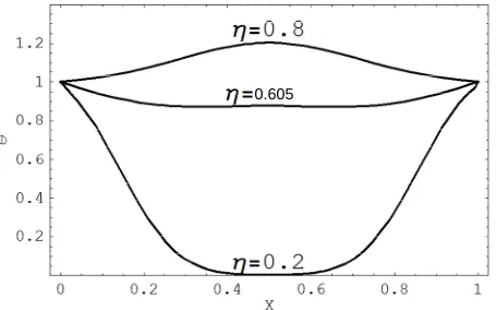
Equation (30b) is plotted using Mathematica program ver. 5. Figure 1 shows the temperature distribution for a thin gold film where the averaging values of the two lag times over nominal range of temperature are q=
11
10 s T = 1013s.
0.605, 0.8
thus with di-
mensionless thickness at dimensionless times = 4.7222 2,
B E
= 1
L
= 0.2,
.
The obtained results show good agreement with those depicted by [1] who solved this problem using separation of variables method.
5.2. Example 2
The objective of this example is to test the proposed Green’s method using heat source and prescribed initial conditions with insulated boundaries. In this example the one dimensional dual-phase-lag heat equation in a thin film subjected to symmetrical time dependent laser heat- ing is investigated by Alkhairy [2] by solving the system
2 3
2 2
2 2
4 2
= 2 ,
B
X X
(31a)
X, 0 = 0,
(31b)
X,0 = 2
X,0 ,
(31c)
0, =
L,
= 0.X X
(31d)
where
X,
= l
X,
r
X,
, (32a)
,
= 0
exp
,l X R
[image:6.595.313.541.83.225.2]0.605
Figure 1. Variation of dimensionless temperature θ for a thin gold film of B = 4:7222E−2; with dimensionless thick- ness L = 1 at dimensionless times η = 0.2, 0.605, 0.8.
,
= 0
exp
r X R L X
. (32c) where R
is the characteristic of the laser beam in-tensity, 0 is the dimensionless capacity of internal
heat source, is the dimensionless absorption coeffi- cient and the subscripts refer to the left and right edges of the film, respectively. In our example, a light heat pulse is adopted, i.e.,
,
l r
= exp
1 .R
(33)where 1 1
= ,
and is the laser heating duration.
Accordingly, the temperature distribution in terms of Green’s function is given in the form
0
source .
exp
, = exp
4
, I C ,
B X
B
X X
d ,
B
(34a)where
source
0 0
1 2
,
, = 4 , 2
, , 2 , , d d
L X
X X
G X X BG X X X
(34b)
1 2
0
,
= 2 , ,0 2 , ,0
,0
I C L
' '
X
G X X BG X X
X dX
(34c)Using Green’s functions from Equations (25a) and (26a) with recognizing that the eigen functions of this example are fn
X = cos
nX
cos
n
LX
witheigen values n=nπ,
L
and the normalization constant
= , 2
n L
N the temperature distribution (34a) can be
written as
0 0
2 2
=0 ,
2 1 1 exp
2 =
cos cos
n n
n
n n
n n
X
L
L
X L X
(35a)where
1
1
2 2
2 2
2 2 2
= exp exp
2
4 sinh
2 4
cosh
2 4
n
n
n
n
A C
A A
A
C
A
(35b) where
1
1 2
1 1
2 =
2 n
C
A
2
(35c)
2
1 1
2
1
2 2 2
=
2
n A
C
[image:7.595.311.542.85.219.2] [image:7.595.55.289.93.469.2] (35d)
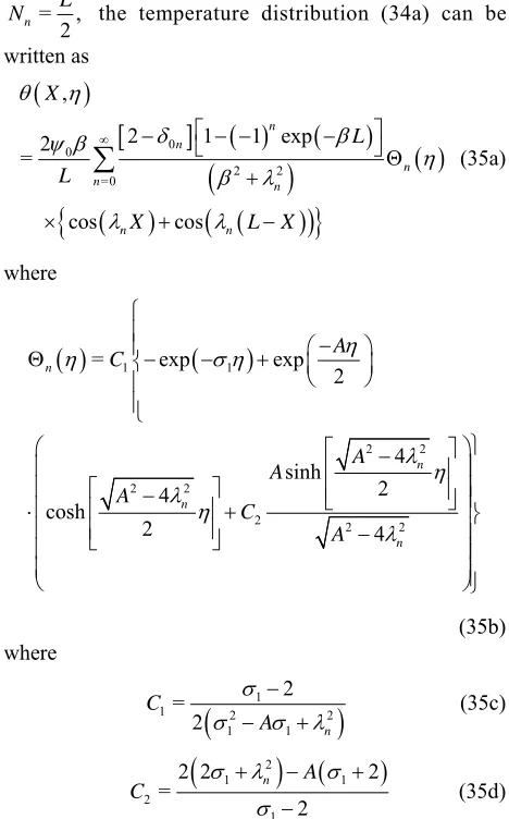
Figure 2 depict the results of calculations of Equation (35a) in a film of thickness for light heat source of dimensionless laser heating duration
= 1
L
= 0.01,
and
dimensionless absorption coefficient = 1 at dimen- sionless time = 0.4, for various dimensionless con- trolling coefficients B= 0.0,0.005, .05.0
With increasing from zero, it is clear that the sharp wave fronts are smoothed and the portions of the disturbance are dissipated. The behavior of temperature response for is called wavelike behavior.
Figure 2 manifests that the wavelike behavior has smaller amplitude of temperature rise than the wavy one
and the increase of results attenuation of the amplitude but not any change in the wide of the por- tion of the thermal disturbance.
B
< 0 0 <B .5
B= 0
BThe obtained results show good agreement with those depicted by [2] who solved this problem using the in- tegral transforms and the variation of parameters method.
5.3. Example 3
Example 2 was also investigated by [3], but for hyper-
0.005
Figure 2. Variation of dimensionless temperature θ for a film of L = 1; η = 0.4; β = 1 for light heat source R(η) = exp
η σ
of dimensionless laser heating duration σ = 0.01.
bolic heat model i.e., . For purpose of comparison, the present Green’s method is applied to the correspond- ing hyperbolic system of Example 2 for instantaneous heat source whose time characteristic of the laser beam intensity
= 0
B
R is given as
=
R (36)
According, the temperature distribution in terms of Green’s function is given in the form
1 0 0
1
=0
, = 4 2 , , d d
, ,0 .
L
X G X X
G X X dX
X
(37)
Using integration by parts and the causality principle Equation (37) can be written as
0 0
, = 4 , , , d d .
L
X X G X X X
(38)Using Green’s functions from Equation (37) with re- cognizing that the eigen functions of this example are
= cos
cos
n n n
f X X LX with eigen values
π
n
= ,
n L
and the normalization constant = , 2
n L
N the
temperature distribution (38) can be written as
0 0
2 2
=0
,
2 1 1 exp
2 =
cos cos
n n
n
n n
n n
X
L
L
X L X
(39)where
Ker , , 0
n n
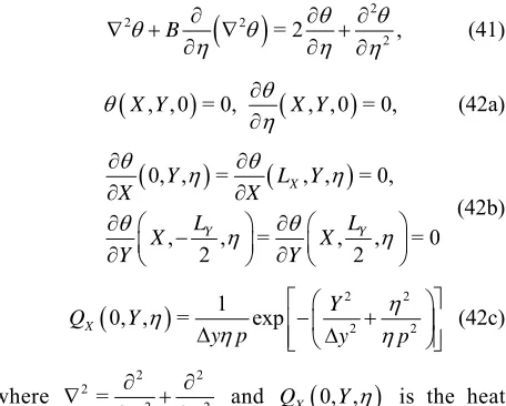
(40)0.9
Figure 3. Variation of dimensionless temperature θ for a film of L = 1; β= 5 for instantanous heat source R(η) = δ(η). (39) for a film of thickness with instantaneous heat source of dimensionless absorption coefficient
= 1
L
= 5,
at various dimensionless times = 0.4,0.9, 2.5.
The obtained results show good agreement with those depicted by [3] who solved this problem using Laplace transforms method.
5.4. Example 4
In this example the two-dimensional dual-phase-lag (DPL) model of heat conduction was investigated nume- rically by [4] for treating the transient heat conduction problems in finite rigid medium under short-pulse-laser heating with Gaussian distributions in both temporal and spatial profiles by solving the system
22 2
2
= 2 ,
B
(41)
X Y, ,0 = 0,
X Y, ,0 = 0,
(42a)
0, ,
=
, ,
= 0,, , = , , =
2 2
X
Y Y
Y L Y
X X
L L
X X
Y Y
0
(42b)
22 221
0, , = exp
X
Y
Q Y
y p y p
(42c)
where
2 2
2 2
= 2
X Y
and QX
0, ,Y
is the heatflux at the boundary Accordingly, the tempera- ture distribution in terms of Green’s function is given in the form
= 0.
X
0
0
=0 =0 1
, , = 2 2
π 2 π
cos cos
n m nm
n m
X Y
X Y
X Y
L L
m X n Y
L L
0.15
[image:8.595.311.539.85.263.2]θ
Figure 4. Variation of dimensionless temperature θ for a finite meduim of dimensions LX = 1; LY = 2 irradiated by
laser pulse with characteristic time ηp = 0.1 and character-istic length Δy = 0.1 with controlling coecient B = 0.0. where
2
1 2
0 2
= 0, , 2 d
y
nm X
y
Q Y G BG Y
d .
(44)Figure 4 depict the results of calculations of Equation (43) for a rectangular medium of dimensions
irradiated by laser pulse with characteristic time
= 1,
X L
= 2
Y L
= 0.
p 1
and characteristic length with con- trolling coefficient
= 0.1
y
= 0.0.
B
The obtained result show good agreement with that depicted by [4] who solved this problem numerically using finite-difference method method.
6. Conclusion
(43)
[image:8.595.60.288.443.626.2]proposed unified method. The obtained results show good agreement with works of [1-4].
7. Acknowledgements
The author would like to thank the scientific deanship of University of Dammam for its generous support of this work through the project No. 2011082.
REFERENCES
[1] M. Xu, J. Guo, L. Wang and L. Cheng, “Thermal Wave Interference as the Origin of the Overshooting Phenome-non in Dual-Phase-Lagging Heat Conduction,” Interna-tional Journal of Thermal Sciences, Vol. 50, No. 5, 2011, pp. 825-830. doi:10.1016/j.ijthermalsci.2010.12.006 [2] R. Al-Khairy, “Analytical Solution of Non-Fourier
Tem-perature Response in a Finite Medium Symmetrically Heated on Both Sides,” Physics of Wave Phenomena, Vol. 17, No. 4, 2009, pp. 277-285.
doi:10.3103/S1541308X09040049
[3] M. Lewandowska and L. Malinowski, “An Analytical Solution of the Hyperbolic Heat Conduction Equation for the Case of a Finite Medium Symmetrically Heated on Both Sides,” International Communications in Heat and Mass Transfer, Vol. 33, No. 1, 2006, pp. 61-69.
doi:10.1016/j.icheatmasstransfer.2005.08.004
[4] P. Han, D. W. Tang and L. Zhou, “Numerical Analysis of Two Dimensional Lagging Thermal Behavior under Short-Pulse-Laser Heating on Surface,” International Jour- nal of Engineering Science, Vol. 44, No. 20, 2006, pp.
1510-1519. doi:10.1016/j.ijengsci.2006.08.012
[5] B. Shen and P. Zhang, “Notable Physical Anomalies Manifested in Non-Fourier Heat Conduction under the Dual-Phase-Lag Model,” International Journal of Heat and Mass Transfer, Vol. 51, No. 7-8, 2008, pp. 1713- 1727. doi:10.1016/j.ijheatmasstransfer.2007.07.039 [6] A. Haji-Sheikh and J. V. Beck, “Green’s Function Solu-
tion for Thermal Wave Equation in Finite Bodies,” Inter- national Journal of Heat and Mass Transfer, Vol. 37, No. 17, 1994, pp. 2615-2626.
doi:10.1016/0017-9310(94)90379-4
[7] F. Loureiroa, P. Oyarzúna, J. Santosa, W. Mansura and C. Vasconcellosb, “A Hybrid Time/Laplace Domain Method Base on Numerical Green’s Functions Applied to Para- bolic and Hyperbolic Bioheat Transfer Problems,” Mec- nica Computational, Vol. 29, 2010, pp. 5599-5611. [8] D. W. Tang and N. Araki, “Wavy, Wavelike, Diffusive
Thermal Responses of Finite Rigid Slabs to High-Speed Heating of Laser-Pulses,” International Journal of Heat and Mass Transfer, Vol. 42, No. 5, 1999, pp. 855-860. doi:10.1016/S0017-9310(98)00244-0
[9] D. W. Tang and N. Araki, “Non-Fourier Heat Conduction Behavior in a Finite Mediums under Pulse Surface Heat-ing,” Materials Science and Engineering, Vol. A292, No. 2, 2000, pp. 173-178.
[10] G. Duffy, “Green’s Functions with Applications,” Chap-man & Hall, New York, 2001.
doi:10.1201/9781420034790