A program generator for designers

FOR DESIGNERS

A thesis

submitted in fulfilment requirements for

of Master of

(Mechanical) in the University of

by A. A. Hunt

CONTENTS

CHAPTER PAGE

AB STRACT .... It ~ . . . 09 ." . . . ., . . . . II) .. II .." . . . . fj . . . It 0 II ill> • 0)" • {O «' . . . \lIO .. ., 0 1

I. INTRODUCTION. . . . 2

II. THE REQUIREMENTS OF A PROGRAM GENERATOR . . . 5

III. EXPRESSING DESIGN LOGIC . . . 7

1. Elements of the design logic 7 2. The global data network . . . 13

3. Designer-control . . . 15

IV. PROCESSING OPTIONS . . . 16

1. Decision tables . . . • . . . 16

2. Data network . . . . . . • . . . 17

V. DATA STRUCTURES . . . . • . • . . . 20

VI. 1. Decision • • • • • • o • • • • • • o e • • • e 20 2., Cases . . . • . . • . • . • . . . . • . . • • . . . . • . • . . . • • 24

3. Trans . . . 26

4. 5. Look-up ts and equations . . . 27

.. " ... 0 *' $ . . . 0' oil • • • • " .. 0 . . . . ., . . . ., . . . . 28

6. Designer-controlled variable lists . . . 29

79 Reset 1 t .. I) . . . 0 ... Go ... 0 e o " • ., • n IJ • • • • • .. .. . . . 29

8. 9. GENERATING 1. Des data elements . . . 30 1 ts "' ... 'Ill iii • • 0- . . . III • • 0 e . . . . e • !It 31

DECISION TABLES AND THE DATA NETWORK 33 program input • • ~uwOooo.e."."G • • • • • 33 2 • sion table input . . o o . w o • • • • w • • oO . . . . I & . i ) 35 3. • • 1 O ( l 9 0 e • • • o • • o • . , 0 . 0 • • • • • 39

6. Entering data into the tory 47 7. Maintenance dependence lists . . . 47 8. Look-up table loading . . . 50 9. Modifying a program • . • . . . 50 VII. DECISION TABLE EXECUTION AND DATA PROCESSING •• 52

1. Recursive execution • . . . . . . . 52 2.

3.

4. 5. 6.

updating ... iii . . . <I- . . . I) . . flO .. e 9 . . . <!l • Ij • (110 . o , 59

Designer-controlled Query / don't query Overriding the value

ab 1 e s .. O' flO .. 0 00 .. . . . 111 63

. . O • • • OOo • • f) . . . 67

a variable . . • . . . . 68 the value of a variable . . . . VIII. IMPLEMENTATION. • • • • • • • • • • • • • • • • • • • • • • • • • • • • • •• 70

IX. DISCUSSION ••••••••• .- •••••••••••••••••••••••••• 78

1. sion tables and program

generator as design . . . 78 2. System developments . • . . . 81

X. CONCLUSION •••••••••••••••••••••••••••••••••••• 89

ACKNOWLEDGEMENTS •••••••••••••••••••••••••••••••••••••••• 90

REFERENCES o • " • • • (Ii . . . «I .. ,. 11 . . . flo • • 0 . . . e .. e «I • ell . . . . " (I 0 . . . ". • • • <& " 0 "Go 91

1

ABSTRACT

A computer-aided design package has been developed which will

enable an engineering designer without conventional computer programming

skills to generate and run a program to be used as a tool in solving a

design problem. In contrast to traditional programs the design system is

based on decision tables, which allow improved documentation,

communication and modification of design logic. Decision tables have

previously been used as a programming medium either as input to a

specialised processor for conversion into conventional program code, or

retained as data to be scanned by a general purpose processor for

checking design constraints. The current package advances the use of

decision tables as data inputs by automating the preparation of decision

table-based application programs. The resulting general purpose

processor is menu-driven and application independent. All program

information, including equations, is stored and used by the system as

data. The Program Generator incorporates both system and design

parameter data manipulation features to maximise the flexibility a

designer is given to control the program logic as well as parameter

values used to reach a solution to a design problem. A worked example on

CHAPTER I

INTRODUCTION

The application of computers as design aids has been wide-ranging in both scope and magnitude. Computer-aided design (CAD) continues to grow, fueled by ongoing developments of both hardware and software packages. While a large number of packages have been written for engineering users, the range of engineering tasks is so great that specialist packages can only provide computer-aid for a comparatively small proportion of frequently encountered uses. To harness the

resources of the computer for tasks for which specialised software is not available, the engineer must either have a package custom developed to his specifications or, in the case of tasks too small or infrequently performed to warrant the expense or lead time of a commissioned program, he must 'write his own software. To write his own programs the engineer must be proficient in computer programming and, furthermore, must be able to justify the time that writing programs requires. Regardless of source, specialised programs tend to be rigidly structured and reflect the style and preferences of a particular designer, thus limiting the ability of another user to choose his own approach to solving a problem. Any changes to program packages needed because of changes in user requirements or source material (such as codes, standards or

specifications) will require further input from a programmer.

design tools by students in the university learning environment. A university teacher setting a problem which requires the use of a computer must either require all students to be proficient in computer programming, or else provide a program into which students can feed their data. Providing a pre-written program will test only the ability

3

of a student to enter data at a terminal, and will not demonstrate his knowledge of the methods required to solve the problem. The tendency to use computer programs as 'black boxes' and automatically accept their output as correct increases the likelihood of failing to detect errors from incorrect data entry or inappropriate assumptions. As stressed by Smith (1986) in a comment considering whether engineering CAD users are "missing the 'big picture''', it important for engineers to be

familiar with methods used in solving a problem. Development of this familiarity and good engineering judgement is important in engineering practice and must be emphasised in the education of engineers. The ideal, then, for the learning environment, is a system which will enable the student to generate a computer program which reflects his knowledge of a solution method rather than of programming techniques. The

reduction of the need for programming skills would make such a system suitable for much wider application in the professional environment.

It is difficult to remove the tendency to use a program from any source as a black box, so it Is important to develop clear documentation of the program method. The inflexibiUty of traditional program

progression from such use of decision tables it would be valuable if the preparation of decision table-expressed application programs could be automated through the use of a general purpose program generator. This would require further development of techniques used to process (run) the generated application programs.

The aim of this project was to investigate the feasibility of developing an application-independent interactive computer package that would enable a designer without conventional computer programming skills to generate and run a program based on decision tables. Such a package would be of particular interest in the university environment.

5

CHAPTER II

THE REQUIREMENTS OF A PROGRAM GENERATOR

Increases in computer availability and usage have not always been matched by system-user interfaces which reflect the widening range of people having direct access to a computer. The primary requirement of the Program Generator is for 1t to provide a CAD tool to engineers who do not have great computer programming expertise. This requires an interactive system capable of informing the user of all its input requirements, whether they be data inputs or instructions. Using pull-down menus of available options is an effective method of giving the user control of the system without needing to key in specific instructions.

There is generally not just a s'ingle solution to a design problem. nor is there often only a single course to a solution. While the design process can be highly formalised the designer will normally exhibit a considerable amount of individualism or art, even if it is exercised within constraints imposed by management policy. standards or codes of practice. The Program Generator must therefore provide a

flexibility of approach to allow the designer to develop and test

alternative solutions within any restrictions which apply. When a design is commenced. not all the requirements of an acceptable solution may be apparent, as some of the restrictions will depend on the form of the design itself. Rather than following a single model right from the

development. Thus, the system should facilitate the formation and

development of computer models with the minimum investment of time or specialised skills. The initial analysis may result in a change of

course in solving the problem in hand and, probably, a refinement of the model in use. Knowledge of the problem may also increase on a broader scale, resulting in changes to codes and standards. Hence, the Program Generator must provide straightfoward updating of logic and design parameters to accomodate progressive development of a particular model as well as influences on the design environment. Ready access to, and control over, the program structure and data input is also required to test the sensitivity of a solution to changes in logic or the values of input parameters.

Ideally, the model expressed in the form of a computer program should be able to be easily communicated to other engineers, whether for checking purposes or for subsequent use or modification.

CHAPTER III

EXPRESSING DESIGN LOGIC

Design of an engineering system is an iterative process comprising two basic aspects: creativity by which the system is proportioned so that the constraints imposed on the system are

satisfied; and analysis whereby system performance is predicted on the basis of a mathematical model. Even though the creative process can be highly individual, computers can still assist the designer in

quantifying his intentions, particularly where the design belongs to a family of similar forms or where there are strong interactions between groups of parameters.

The Program Generator is built on the conceptual framework provided by Fenves (1972). The terms' 'ingredlence' and 'dependence'. used here to express the relationships within the design logic network, are from the same source.

1. ELEMENTS OF THE DESIGN LOGIC NETWORK

The design logic network is made up of inter-related data elements. The basic relationship between the data elements may be described as a transformation (Fenves, 1972) Ti, of the form

where:

Ti : Yi ::::: fiIt(y!)

Ii ::::: (xu, Xu!, ... Xin),

Yl is an output variable, Xij are input variables,

f is a functional relatIonship between input variables.

The transformations Tn may take the form of functions or logical decisions, and may be based on proven theory or subjective opinions. Individual Xin may be called ingredients of Yi and, hence, h. the collection of ingredients, may be called the .:!:.!:.!.I~~~~.!..!!:!~

of yt. Conversely. as the value of Yl depends on each Xu on its ingredience list Ii, Yi may be called a dependent of each Xln. An

input variable may be a ingredient of more than one output variable and have more than one dependent. The collection of all the dependents of an input variable Xik may be called the dependence list of Xlk,

D(Xi) (Yilt Y12 .... Yim)

For example, a direct stress, Sd,might be calculated from the applied force, F. and the cross sectional area, A. F and A are thus ingredients of Sd, and Sd is a dependent of both F and A.

The value of Yl may be determined by one of a number of functions; the relevant function is identified by the logic of the

problem and each function has its own set of ingredients. For example, the support and loading conditions of a beam determine which function used to determine the bending moment.

9

When a design problem is computerised, flow charts are commonly used to describe the program logic. However, the flow chart becomes unwieldy and confusing with large or complex programs and is not readily updated. Like flow charts, the derived programs are often inflexible and have poor readability, with reliance placed on the programmer to provide sufficient documentation. These factors may make the system production and maintenance costs higher than the costs incurred in actually running the program.

Decision tables which express the design problem's logical

conditions, possible actions, and the logic linking the two in a tabular form are an alternative to flow-chart based programs and documentation. Decision tables are more readable and concise than flow charts, hence relationships between variables are more readily apparent and may be easily updated and maintained.

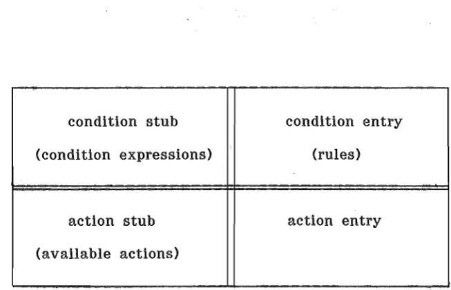
condition stub condition entry (condition expressions) (rules)

action stub action entry (available actions)

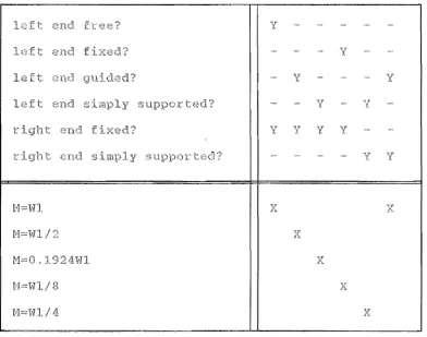
A decision table consists of four parts as shown in figure 3.1 and a sample decision table is shown in figure 3.2.

The condition stub lists the logical conditions on which a decision is based. The action stub lists all the actions which may be taken as a result of the decision. An action might, for example, be the assignment of a value to a variable (eIther directly or through the application of a particular equation) or the execution of another

table. The _condition lists all of

f1: end f

lE;1ft gu

left s1mply upported? y

r end f ? y y y

t ,,~nd y suppo:rt(",d

x

bendin.g m0n12rl

fore :Lnt load

1 1

the values of the logical conditions in columns. Each column of the condition entry is called a 'rule'. The elements of the condition entry may be Y (yes), N (no), or - (immaterial). (Some texts use Y. N. and I, respectively.) The action entry indicates the actions to be taken should each particular rule apply. Action entries may be X, indicating that the action in the same row of the action stub as the mark is to be carried out, or blank if the corresponding action is not to be carried out. (Some texts use Y and blank. respectively.) Decision tables using only y, N, and - (or their equivalents) in the condition entry are called limited entry tables. McDaniel (1968) gives further information on extended entry tables.

11

In any given situation only one decision table rule may apply but any number of actions may be executed as an outcome of that rule.

In situations in which more than one rule fits the state of the condition stub the table is said to be ambiguous (Fenves, 1966). As table rules are scanned from left to right for an appropriate rule the left-most rule that fits applies; any subsequent rules are not examined.

A decision table is said to be complete if rules are stated for all combinations of the logical variables in the condition stub.

-(immaterial) or may be implied by a processing algorithm with the ability to detect a 'no rule applies' state.

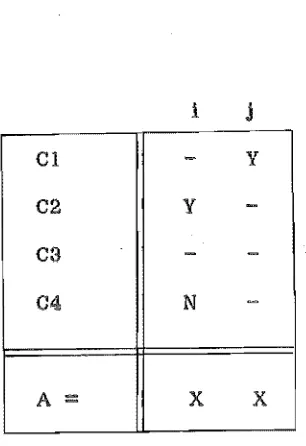
Dependence relatIonships can arise through logical as well as functional transformations as shown in figure 3.3.

With repect to figure 3.3, data element A is dependent on conditions 02 and 04 if rule i applies, and on condition 01 if rule j applies. Element A is not. however, a dependent of 03 as both entries in row 3 are immaterial.

1 j

01

-

02 Y

-03

-04 N

-A

=

Figure 3.3 Dependences from logical relationships.

The advantages of decision tables to describe design logic can now be better appreciated. Firstly, the logic which applies to a

13

the completeness of the table can be readily assessed and any

ambiguities or other errors identified. Secondly. unlike the flow chart,

additions and alterations do not alter the clarity and compact nature of

decision tables. This provides a distinct advantage in applications such

as computer program documentation where accurate communication of the

design logic is essential. Thirdly, decision tables can be easily read,

analysed and written by non-computer programmers more readlly than can

flow diagrams. Fourthly. the standard layout of decision tables offers

the potential for formalised preparation and processing, including

direct use as a programming language. These characteristics,

particularly the latter two, are the major reasons for using decision

tables as the basis for the Program Generator For Designers.

2. THE GLOBAL DATA NETWORK

As an output variable from one transformation· may in turn serve

as an input variable to another transformation, supplying the

ingredience list for each element provides sufficient information to

completely describe the data network.

Two wider relationships can now be identified: the global

ingredience and global dependence of a data item. The global ingredience

of a data item consists of all the data items influencing it. its

ingredients, the ingredients of its ingredients, and so on. Global

ingredience is obtained by traversing the network from right to left

untll all the data elements which may be accessed have been reached. The

global dependence of a data item consists of all data elements depending

until all the data elements which may be accessed have been reached.

2

M bending moment

SATISFIED if level 1 :::: TRUE

o

Y distance N.A to farthest fibre

I second moment of area

R f'eelction fo",'ce

F appl

x dis

br"ecldth bea,n

beam from support )

Data network for a simply supported rectangular beam

15

With respect to figure 3.4, each element on the network can be described as being a certain level from output. As a data element may be an ingredient to a number of dependents the level relative to each

particular output may be different, hence within the global network Fenves (1972) defines the global level from output as being that which gives the longest path from the particular data item to any output item.

3. DESIGNER-CONTROLLED VARIABLES

Within the network there exist input items which have values controlled directly by the designer: these will be refered to as

CHAPTER IV

PROCESSING OPTIONS

1. DECISION TABLES

Once a design problem has been expressed in decision table form there are two options for use of decision tables as programming aids. The first is to convert the decision tables into a conventional

tree-structured program, either manually or by using a programmed preprocessor. More than one tree-structured program can be derived from any particular decision table depending on the sequence in which the programmer chooses to arrange the design condition expressions from the condition stUb. The second option Is to retain the decision table in its original form, store it as data, and use it as input to a general

purpose interpretive program. This sec-ond approach offers greater flexibility than the first, as updating or altering the problem logic does not affect any of the interpretive routines. The tree-structured approach offers a potential basis for a program generation strategy, assuming that a computerised preprocessor is used, but it lacks flexibility and requires considerably more processing programs of

greater complexity than does retaining the decision tables as data. The 'store-and-use-as-data' option has the added advantage of neatly fItting in with strategies for storing and using the elements of the wider data network.

processor is that the clarity of logic provided by decision tables renders the additional computer program documentation required by conventional programming methods unnecessary.

2. DATA NETWORK

To execute a decision table one proceeds from a given set of input data. evaluates the logical variables of the condition stub, and then carries out the actions indicated by the appropriate rule. As the set of input data will not contain all the information required to

complete execution. some strategy is required for the evaluation of this other data. To overcome this problem 'direct' or 'conditional' execution may be used.

Direct execution reflects traditional flow chart program layout which requires data to be arranged and processed in a predetermined order. Execution begins with the input data and moves 'bottom-up' to derive data at higher levels from input. Execution halts if any data item encountered is not defined at the time it is required. In terms of the network illustrated in figure 3.4, the data network must be

evaluated from left to right.

Conditional execution leaves the computer program to decide the sequence the process follows according to what data is or is not defined at the time. This 'top-down' logic allows execution to begin even if some ingredient data is not defined. Thus. if while evaluating some data item it is found that an ingredient of that item is also not defined, processing of the the first item is temporarily ,suspended. while the

second is evaluated, and is then resumed.

The conditional execution approach has several advantages over

the direct approach:

1. Immaterial condition entries in a decision table mean that

not all conditions may need to be evaluated for the

decision table to be executed. Under some circumstances it

may not even be possible to supply a complete set of input

data.

2. Optional data, which may remove the need to evaluate some

lower level data, is more readily accomodated.

3. Any updating or correction of design constraints or other

data requires little effort compared with the possible

reprogramming and compilation required if a direct

approach is adopted. This is of particular importance

within an interactive program generation strategy where

maximising the 'user-friendliness' of the system requires

that such alterations be easily achieved.

4. The most natural sequence is 'top to bottom' in line with

the logic of the problem itself as reflected in the

ingredience lists. Hence, once a problem is expressed

within the framework outlined in Chapter III, conditional

19

CHAPTER V

DATA STRUCTURES

The relationship between decision tables and stored data is shown

in Figure 5.1. The names of storage areas shown are those used by the

program system programs for the equivalent arrays. A leading 'N' is

often used in a name to indicate an integer array or variable to the

system programs which use FORTRAN implicit naming conventions.

1. DECISION TABLE STORAGE

Figure 5.2 is complementary to figure 5.1 and represents the

detail of the stored decision table.

Condition and action stubs are" not stored in their original form

by the system. The condition stub is used to store pointers (NSTORE)

which indicate the storage locations of the state of each of the

conditions (arrow 1, fig. 5.1).

The action stub is used to record the type of action (NTYPE), the

number of the equation to be used if the action type specifies

DIRECT

RLKDAT

CALC

7.

Note: for key to arrows see fig.5.lb

5.la

r

NEQN,L NTABD, NAME, UNITS, NDEPN

- - - 1 - - - - . 1

i

NDCV

8

MESAGE

.1:\')

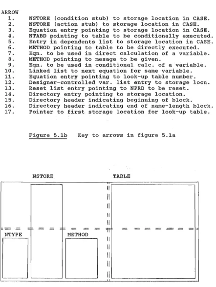
ARROW 1. 2. 3. 4. 5. 6. 7.

8.

9. 10. 11. 12. 13. 14. 15. 16. 17.

-

-NTYPE

NSTORE (condition stub) to storage location in CASE. NSTORE (action stub) to storage location in CASE. Equation entry pointing to storage location in CASE. NTABD pointing to table to be conditionally executed. Entry in dependents list to storage location in CASE. METHOD pointing to table to be directly executed. Eqn. to be used in direct calculation of a variable. METHOD pointing to mesage to be given.

Eqn. to be used in conditional calc. of a variable. Linked list to next equation for same variable. Equation entry pointing to look-up table number. Designer-controlled var. list entry to storage locn. Reset list entry pointing to NPRD to be reset.

Directory entry pointing to storage location. Directory header indicating beginning of block.

Directory header indicating end of name-length block. Pointer to first storage location for look-up table.

Figure 5.1b Key to arrows in figure 5.1a

NSTORE TABLE

II

II

II

II

II

::: - - ₌₁₌

-

-9f - - - -

-

-METHOD

"

II

II

II

location of any variable required (NSTORE). Actions are restricted to four types:

23

1. Calculation of a variable (NTYPE :::: 1). As the method of calculation of a variable may vary from one application to another, a variable cannot be retricted to association with only one equation (e.g. the equation for the bending moment in a simply supported beam is different from that for a built in beam). Array NSTORE holds a pointer

indicating the storage location of the variable which is to be calculated (arrow 2, figure 6.1), while METHOD points to the equation to be used in the calculation (arrow 7, figure 6.1).

2. Displaying the value of a variable (NTYPE .= 2). The

storage location of the variable indicated by NSTORE. No method is indicated as the action requires the current state of the variable to be displayed.

3. Direct execution of another decision table (NTYPE .= 3,

NSTORE :::: null). A pOinter (METHOD) indicates the decision table which is to be executed (arrow 6, figure 5.1).

These modifications to the condltion and action stubs are made by the system programs after the decision table has been entered. Condition and action entries are stored in their original forms.

2. CASES

The values of data elements (including condition stub members) are stored in the array CASE. Storage locations start at address 51 as mathematical operations are numbered from 1 to 35 and look-up tables are numbered from 36 to 50. Associated with each storage location is a

PResence of Qata flag stored in NPRD.

Presence of data are normally boolean status indicators. The status of a data element is valid (NPRD = 1) if it has been calculated using the current value of each of its ingredients (Le. presence of data flags for each of its' ingredients are set to valid). The status of a data element is void (NPRD

=

26

which is a member of the overridden variable's global ingredience, any valid data elements (Le. NPRD :::: 1) in the global dependence of the altered designer-controlled variable would, in the normal course of events, be set to void (NPRD =: 0) thereby defeating the object of the

override in the first place. Hence, when the value of a data element is overridden its presence of data flag is set to '2' (NPRD :::: 2), even though its status for use in the calculation of its dependents is effectively set to '1'.

Multiple sets of NPRD and CASE are stored, allowing a case study approach to the design process whereby the designer may use one of a number of sets of data. Storage locations are the same for each list so other information, such as the dependence list associated with each location, does not require multiplication. Different case studies can be reserved for specific purposes, such as standard base data, or for use

•

by different system users or to record- successive design iterations for future reference.

After an existing case study is selected, its contents are copied into case study 1, which is reserved as a work area, leaving the

and start again with a fresh copy of the original data.

In this project the number of case studies has been arbitrarily

set at six including the work area.

3. TRANSFORMATION AND DESCRIPTIVE DATA

When a data element is to be evaluated by execution of a decision

table, the TABle Qesignation NTABD indicates the decision table to be

used (arrow 4, figure 5.1). If a data element is to be calculated

directly from its ingredients, the equation whose number is stored in

NEQN is used (arrow 9, figure 5.1).

When the value of a data element is to be determined, NTABD is

checked first and if it is non-zero the indicated table is executed. If

no table is indicated and NEQN is non-zero, the indicated equation is

used for direct calculation (arrow 9, figure 5.1). If both NTABD and

NEQN are zero then the element is a designer-controlled variable whose

value must be assigned directly by the designer.

In cases where both NTABD and NEQN are non-zero the indicated

decision table is executed; the equation number is only significant

during the input of the data network structure. This will be detailed in

Section 4 of this chapter.

There are two sets of descriptive data associated with each

storage location. NAME stores the variable name, which for a condition

units in which the value of the variable is to be entered. Units are descriptive only and a unit compatibility check is not made by the system

4. INGREDIENCE LISTS AND EQUATIONS

27

Pure ingredience list are not stored or used by the system as they are implied in the equations supplied by the designer. Two forms of each equation are stored in CALC: the raw form, as entered by the

designer, and Its Reverse Polish form. The raw form is retained for the benefit of the designer in case it is required for viewing or editing. During processing of the raw equation. operators are replaced by a code number in the range 1 to 30, variable names are replaced by pointers indicating a storage location (arrow 3, figure 6.0 and look-up table names are replaced by a look-up table number in the range 36 to 60. Spare code number slots are available" if future designers wish to insert custom operations. The first element of the processed list tells how many elements are in the list. When a look-up table number is encountered during execution, the table number gives access to the starting address in the storage array RLKDAT, and the table arguments combined with other data allow the actual data location to be

identified.

To enable all the equations associated with any particular data element to be identified, the equations are linked using a linked list format with the first equation indicated by NEQN (arrow 9, figure 5.0

run-time when decision tables are used to decide which is the appropriate equation to use (arrow 7, figure 5.1).

The convention used in the Program Generator, when storing lists of data such as processed equations, is to use the first entry in the storage area to indicate how many entries are in the list.

5. LOOK-UP TABLES

Look-up tables provide a user-defined array-type data storage facility which is intended for use when the designer would otherwise have to refer to tables of standard or other reference data. During

execution look-up tables are read only, their values having been entered by the designer during the program input phase. A total of 15 look-up tables may be created.

In the Reverse Polish form of an equation the pointers indicating the storage locations of the look-up table arguments are encountered first, followed by the number of the look-up table itself. Data for all look-up tables is stored in sequence in the array RLKDAT. LKPTR holds pointers indicating the starting position within RLKDAT of each look-up table (arrow 17, figure 5.1). LKDIM gives the number of axes of each table and is used during the running of a program to check that the correct number of arguments have been included in the equation

29

LKNAME look-up table name

LKDIM number of axes or arguments associated with the table LKSIZE number of entries along each axis of the table

LKAXIS name of each table axis

LKTOT total number of entries in each table

LKPTR pointer to the starting location in RLKDAT for each table

LKNEXT pointer to the next input slot in RLKDAT to be used by a new table

6. DESIGNER-CONTROLLED VARIABLE LISTS

Associated with each decision table is a list of

designer-controlled variables, NDCV; the value of each of these variables may be changed before the decision table is run. The list format the same as that for dependence lists, with pointers listed instead of data element names (arrow 12, figure 5.1); the first element in the list gives the list length.

The same designer-controlled variable will occur in more than one list if it is in the global dependence of more than one condition

expression, but because NPRD is set to 'valid' after the first query of its value the designer wlll only be queried once per program run.

7. RESET LIST

funning of an application program, a pointer indIcating its storage

address in CASE is added to the reset list NRESET. This records that the variable's presence of data flag, NPRD, has been set to 'valid' after the designer was given the option of changing its value. At the

completion of the run the presence of data flags at all addresses on the list are reset to 'void' (NPRD ::::: 0), so that the system will give the designer the option of changing the value of the variable during the next program run, and the list length Is zeroed.

Pointers indicating the storage locations of overridden variables are also stored in NRESET so that the variable is restored to its normal status after the completion of the design program run.

Unlike the other data structures which have been discussed, the state of NRESET is dependent on the running of the application program rather than on its generated structure. As the list is zeroed after each program run is completed it exists only in memory and is not permanently stored.

8. DIRECTORY OF DATA ELEMENTS

The data storage areas discussed thus far use storage addresses instead of variable names as a reference. The link between names and storage addresses is provided by the ordered directory DIRECT which documents data element names and their corresponding storage locations. The directory is ordered firstly on name length and secondly on

of the block corresponding to each name length as is illustrated by arrows 16 and 16 in figure 6.1. Arrow 14 in figure 6.1 illustrates the link between DIRECT and CASE.

9. DEPENDENCE LISTS

In figure 5.1. dependence lists are shown stored adjacent to the storage location of the data element to which they pertain. The

dependence lists, instead of listing dependents names, contain pointers indicating the storage location of the element on the list (arrow

31

figure 5.1). The first element of the dependence list tells how ,many pointers follow in the list. Associated with each entry in a dependence list stored in NDEPN is an equation number stored in NSORCE. The

equation identified in NSORCE is that which gave rise to the dependence. The NSORCE equation number is used by the WARN3 algorithm detailed in Chapter VII, to determine whether the" associated dependence relation recorded by NDEPN applies at a particular time.

As was outl1ned in Chapter III. dependence relationships can arise from the decision tables themselves. A change in the value of a condition stub expression can change the rule which applies and, hence, the values of any relevant action stub expressions (see figure 3.3). To enable these relationships to be traced during the running of an

application program, dependence lists are also used to record dependent decision tables. If it was not for the decision table, a condition

table number to be distinguished from a variable storage address, lists of dependent decision tables, associated with condition expressions, start with a leading zero and the second entry in the storage area gives the list length, the remaining entries are the dependent table numbers. Thus, the global dependence of a data element can be traced, any

33

CHAPTER VI

GENERATING DECISION TABLES AND THE DATA NETWORK

The suite of algorithms associated with the program generator can be divided into two functional groups: the first for design program

generation; the second for running the generated program. A third function, that of modifying the generated program, selectively uses all or part of the algorithms developed for program generation and so will not be considered separately.

The purpose of this chapter is to discuss the algorithms developed for design program generation.

1. DESIGN PROGRAM INPUT

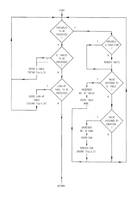
The parent algorithm for program input is DESPGM, illustrated in figure 6.1. Execution of the algorithm is triggered when the design selects the 'enter a new program' option within the calling algorithm which then increments the number of decision tables by one and calls the DESPGM routine. Execution is repeated until the new decision table, and any subsequent decision tables and all resulting variables and look-up tables have been entered. The algorithm is structured so that all

ENTER D. TABLE

(DETAB fig.6.2l

Figure 6.1

START

y

N

RETURN

NO. Of -ABLES

,

NAME

y

REQUEST UNITS

N

Y VALUE ASSIGNED BY

EQU/mON

INCRE ~ENT ?

NO. Of EONS

• N

ENTER EQN

!

PROCESS EQN

ENCODE (fig.6.3)

it is the system which decides the order in which decision tables and

equations are entered and the designer is prompted accordingly. This is

made possible by the processing strategies adopted and the resultant

data storage methods. The data input process can be viewed as a series

of partial traversals of the developing data network from right to left,

with each traversal being completed when all the data downstream from

each decision table is allocated storage.

2. DECISION TABLE INPUT

Figure 6.2 represents the DETAB algorithm for decision table

input. Parts of the subroutine built on this algorithm are also used

when additions or alterations to decision tables are required.

As part of the processing of condition stubs, dependence

relationships between decision tables and conditions are noted by

recording the decision table number in the dependence list of each

condition stub expression. This information allows potentially affected

decision tables to be identified when, during the running of a design

program, changing the value of a variable affects all elements in its

global dependence.

During processing of actions which call for calculation of a

variable, the algorithm calls for entry of units for the variable and an

equation for use in calculation of the variable. This may, at first,

appear to duplicate parts of the DESPGM algorithm of figure 6.1,

however, within DESPGM the variable is calculated directly from its

ingredients whereas within DETAB provision must be made for selecting

'I

+

ENTER NUI'18ER

Or: CONDlnON~)

,

ENTER NUI'16ER

OF ,~CTli)N;)

,

Of RULES

•

FIRST CONDITION

! ..

•

CilEeK 1,IHETHER

CC'NDITION KNO~IN

(INDEX fig 6.7.1

PROCESS CONDITION

AS AN EQUf\TION (ENCODEf,ig 6.3)

CiECORD DECISION TAl:,U: CONDITION DEPENDENCY

ENTRY OF

i\CTIOW3

(f ig. f;" 2b)

t

E~ITRY OF'

RULES (fig. i).2c)

~

N

y

FOR VARIABLE

LIST ALL EXISTING EQUA nONS FOR CALC. OF VAR.

I

SELECT EOUA nON

Y

INCREMENT ?

NO. OF EONS.

I

ENTER EQUATION

I

PROCESS EQUATION (ENCODE fig 6.31

Y

37

STr

FIRST ACTION

~Nm

SELECT ACTION TYPE

?

N

ACTION IS DISPLAY A

MESSAGE

t

DISPLAY LIST OF MESSAGES

N y

DISPLAY LIST OF EXISTING TABLES

I

SELECT TABLE

INCREASE NO. TABLES

I

REOUEST TABLE NAME

Y

ENTER MESSAGE

ENTER VAR. NAME

I

PROCESS VAR. NAME (INDEX fig 6.71

N

END - - - ! I ! - - - < .

START

t

ENTER RULE

END y

6 2c Algorithm DETAB.

"

-NEXT RULE

from a range of equations, the choice depending on the conditions which will prevail at the time of its use. Hence, the equation must be

identified at this point and units are recorded at the same time.

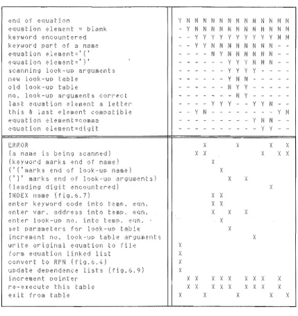
3. EQUATION ENCODING

As an input equation is scanned using the ENCODE algorithm of figure 6.3, a second (temporary) equation is built up of operator codes, variable storage addresses and look-up table numbers instead of the names and symbols used originally. A list of codes is shown in figure 6.4. The key part of the algorithm is the use of a list of standard keywords such as operators ('+', '-', etc.), trigonometric and

logorithmic functions ('sin(', 'log{' etc.) and digits ('O' to '9'). 'l'he

use of various checks allows identification of the embedded variable and look-up table names. If pi, yes, no, true or false are identified as

keywords, a check is made whether it· should be identified as such or if

it is part of a variable or look-up table name.

Unlike a programming languages such as FORTRAN, the ENCODE algorithm allows embedded blanks within look-up table and variable names. This ellminates the need to eliminate the need to link separate words in one name, for example by underscoring, thereby eliminating a potential source of error for a novice user.

39

Neither leading digits in names nor numbers are allowed within equations. Instead of using a number the designer must use a variable to which the appropriate value is assigned during the funning of the

en of qual: i ':"in Y N N N N ~I N N N N N ~I ~I N quat ion lem nt blank Y N N ~I ~I N ~I N N N N ~I N

keywor'd n OLlr1t ered '{ Y Y Y Y Y Y Y Y Y N N

keYi~ord par of a name Y Y N N N N N N N ~I

equation e eml.:'nt , ( , -

-

--qLI t on element ' ) , y y y _{N N} N

s nning look-up argLlments - Y Y Y Y

-new look-!JP table -- - y _{N N} - - _-

-old look-up table ~I Y Y - - - -

-no. look LIP rgument rrect

-

--

-

-last eClLlation element 1 tter Y Y Y

-

this & 1 (:1 s t e1 m nt compatible Y N -- -- -. _-- y ~I

tion element mma -- Y ~I N

element dig it - -- ," y y

Ef~fWR X X X )(

( ;oj nam b in0 so nn d) X X v }\ X X

(keyword marks ·",nd of n In v 1\

( , _{('marks end of look}

UP name) X

( , ) , _{marks end l')ok-up ar Lim nts) X X}

(1e ding dlgi encounterE'cd) v

A

INDEX nam (fig.6.71 X X

enl;er k yl}}ord code into t ,emp" eqn. X X

enter var. address. nto temp, eqn, K X v

l\

nter look-LIP no. into temp. i;;·qn, X

parameter or look-up table' '/

J\

in remen1: no. look-up tabl rguments X

I,wi e ori<;lin 1 e uation to file X

Qrm eq!.! tiOil linked l i t X

convert to RP!~ (fig.6.4.) X

upclat d pen de nee list (1'18,6.9) X

increment point.~r X X X X X X X v X

"

r -·,,:xecute thi table X :< X X X X X \I _X

)\

ex t i'rom tab X X X X V

i\

41

Symbol Code Symbol

=

<: 2 LOG( 19

>

4. 0 21

5 1 21

+ 6 2 21

**

9 4 21

*

/ 8 6 21

10 7 21

11 8 21

SIN( 12 9 21

COS( 13 TRUE 22

TAN ( 14 FALSE 23

ASIN( 15 YES 22

ACOS( 16 NO 23

ATAN( 17

Note: during equation other characters use code 33

automatic querying of designer-controlled variables during each run may be suppressed. This strategy was adopted to avoid the complications of having to assign a numerical value to a character substring consisting of digits. which may have been expressed in different but numerically equivalent forms.

A checking matrix is used to check the compatibility of adjacent equation elements, e.g. a variable may not follow a close bracket ')'.

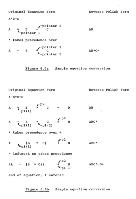
4. CONVERSION TO REVERSE POLISH NOTATION

The ENCODE algorithm encodes the raw equation into a numerical form with elements in the same order as the original. The RPN algorithm of figure 6.5 retains the numerical form but reorders the equation into Reverse Polish notation. Some sample conversions using RPN are shown in figure 6.6 which retains the original symbols for simpUcity.

The RPN algorithm is based on a scanning of the preprocessed equation using up to two active pointers at anyone time. Pointer 2 is the leading pointer and is incremented along the preprocessed equation, whereas pointer 1 is a marker to be inserted where and when required. Variable addresses are put into the Reverse Polish equation as they are encountered by pointer 2. If pointer 2 encounters an operator, pointer 1 is inserted. and the incrementing of pointer 2 continues. If

43

pointer at var abl address Y N N N N ~I N ~1 N ~1 ~I N N pointer " _{al: nel of quat ion Y Y N ~J N N N N N N N N}

"

pointer' 2 at t'i gh br cket ' )' - - y y y y _{N N N N ~I ~I}

pointer' 1 activ ~: this level - Y Y Y N Y N N Y Y Y Y

1 ve1::1 '( N ~I N Y Y

pointer at OP rCl tr)r ~ Y Y Y Y '( Y

0 neer 2 at comm

-

p r tion at f}oint r2 takes pr',~cedence N Y Y Y

po 1 at - & pointer at + Y

-po _at ;4(

& pointer '2 at / - - - - y

put element at point r' '2 UHO RF'N eqn X

p t r-l (this level) l,~ III nt into RPN qn X X X v _{X X}

j\

d activate point r' 1 ~ _{this 1 ,:';v e 1 X X}

X :~ X X X

l,

tack, incr'<?ment 1 v X

tiv

ce

un t; ck, d cremen 1 v 1 v X v _{X X X X X}

-~

"-n r' in nl: point(~r' X ;< v r, X X X v J\ X X

r x cute this tabl X X v _{,', X X X X X X X X} v _A

xit thL:; table v

1\

~I 0 'cf: : pointer 1 .-:;. x i _{t t dif} r' nt 1,,: V _{t IX}

r-' 'ferences t () oint: r 1 apply to til urr nt lev L

Original Equation Form A*B-C

rpointer 2

*

A

\"'pointer 1

'* takes precedence over

-A B

,pointer 2

- C

"'-pointer 1

Figure 6.6a

Original Equation Form A-B*C+D

r

A - B

'*

'L

A - B

It.p1 (1)

'*

+

*

r

D

D

A - [B 11 C]

It.p1 (1)

+ D

- leftmost so precedence

(A

,p2

+ D

[B

'*

Lp1 (1)

end , + entered

6.Gb Sample equation

Reverse Polish Form

AS

AB*C-conversion.

Reverse Polish Form

AB

ABC*

ABC*

in figure 6.6b, the operator at pointer 2 takes precedence, it cannot immediately be entered into the equation in case there is a third

45

operator which takes precedence over the operator at pointer 2. To allow this, stacking occurs: the position of pointer 1 is stored at 'levell' and the working level is increased from 1 to 2. Processing continues ignoring pointer 1 (at level 1), as if the operator at pointer 2 was the first operator encountered. A new marker, pointer 1 (at level 2) Is then inserted at the position of pointer 2 and scanning continues. When the +

(addition) is encountered, ,. (multiplication) takes precedence and Is entered into the equation. Unstacking then occurs: pointer 1 (at level 2) is deactivated, and operation resumes at level 1 where the original pointer 1 Is reactivated. A comparison is then made between + at pointer 2 and - (subtraction) at the reactivated pointer 1 (at level 1).

Addition has a higher valued code but a separate check for equal precedence operators occurring at the two active pointers (Le. - or It

at pointer 1 corresponding to + or I respectiVely at pointer 2) enters the left-most of the two operators, -, into the equation, followed by

the addition operation when pointer 2 encounters the end of the

equation. Thus, only one pass of the preprocessed equation is required to build up the new equation in Reverse Polish form.

6. INDEXING OF DATA ELEMENTS

The directory DIRECT accessed by the INDEX algorithm which conducts a linear search of the appropriate name-length block to check whether the variable name given to it by the calling algorithm exists.

~

REMOVE LEADING BLANKS

I

REMOVE TRAILING BLKS

~

LOCATE BLOCK OF SAME LENGTH NAMES

I

FIRST NAME IN BLOCK

1 - - -... -NEXr NMlE - - - ,

y

RETURN - - - 0 1 I I I I - - - <

RETURN - - -... 111---MESSAGE 'NOT FOUND'

F

N

DIRECTORY

?

Y

ENTER NM1E (INSERT fig.6.8)

j

A19'Jri thm INDEX

47

directory the algorithm can be used to mark the position where the name

would be stored if it were to be entered into the directory, for

instance during the scanning of an equation.

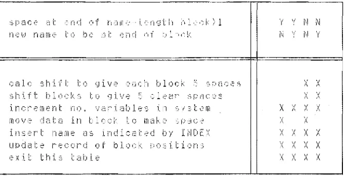
6. ENTERING DATA ELEMENTS INTO THE DIRECTORY

When INDEX determines that a new variable name Is to be added to

the system, the location which the new data is to occupy in the

directory is passed to the INSERT algorithm (figure 6.8) which

manipulates the data in DIRECT. If the space between the target block

(the block corresponding to the length of the new name) and the

following block Is insufficient, the algorithm checks the space between

all adjacent blocks and moves them within the storage area so that there

will be five clear spaces between blocks after the new name is inserted.

This reduces the frequency of directory data shifts.

7. MAINTENANCE OF DEPENDENCE LISTS

After an equation has been encoded (using ENCODE) and converted

to Reverse Polish notation (using RPN) it is processed by the algorithm

DEPLST which maintains dependence lists. Feeding DEPLST an equation

gives it the same information as would feeding it an ingredience list.

To maintain dependence lists, the subject of the equation needs to be

added to the dependence list of everyone of its ingredients. Hence,

DEPLST consists of two nested loops: the outer to scan the equation for

variable addresses and the inner to scan the dependence list of each

variable address in the equation and add the target variable address to

space at nd of nam -length block>l Y Y ~I N new nam to be at end of bl ck ~I Y N Y

calc shi ft to give each block 5 spaces X X

shift blocks to give 5 clear spaces X X

increment no. variables in system X X X X

move data in block to mak pace X X

ins rt name as indicated by INDEX X X X X

update record of block position X X X X

xit thi table X X X X

N

1---

y

N

START

~

1ST ELEi1ENT IN NEW EON

EWIENT VALUElSO

?

y

READ IN DEPENDENCE LIST OF EON ELEMENT

I

1ST DEf. ON LIST

LIST

?

y

ADD TARGET ELEMENT TO DEPENDENCE LIST

?

y

END

Note: the 'target ~lement' is the LHS of the new equation N

NEXT DEPENDENT

ON LIST

9 Algorithm DEPLST

When equations are modified they are reprocessed by ENCODE, and

DEPLST is then re-run. If any variables have been removed from the

original equation a routine UNDEPN removes the subject of the equation

from the dependence llst of the ex-ingredient.

8. LOOK-UP TABLE LOADING

Algorithm LKLOAD, illustrated in figure 6.10, interactively

loads the designer's tabulated look-up data into the storage area

RLKDAT. Up to five table axes can be accomodated and, after loading the

axes' descriptions and lengths, five nested loops control the loading of

data elements into successive slots in RLKDAT.

9. MODIFYING A PROGRAM

A generated program can be readlly edited or expanded by a

'modify' option which makes selective use of the algorithms discussed

START

t

1ST TABLE AXIS

ENTER AXIS NMIE NEXT AXIS

~

ENTER AXIS SIZE

N

?

y

RECORD TOTAL NO. OF TABLE ENTRIES

TO LKTOT

t

RECORD NEXT SLOT NUMBER IN RLKDAT

TO LKNEXT

t

END

Figure 6.10

51

FIRST ENTRY ON AXIS 1 FIRST ENTRY ON AXIS 2

FIRST ENTRY ON AXIS 3

FIRST ENTRY ON AXIS ,

FIRST ENTRY ON AXIS 5

ENTER LOOK-UP TABLE ENTRY INTO RLKDAT

N LAST ENTRY NEXT ENTRY~f---<

N LAST ENTRY NEXT ENTRY """"'1--<

N

NEXT ENTRY .... -<

N

NEXT ENTRY

N NEXT ENTRY

Algorithm LKLOAD

LAST ENTRY AXIS .3

?

?

CHAPTER VII

DECISION TABLE EXECUTION AND DATA PROCESSING

The algorithms associated with running a generated application program fall into two groups: those which actually run the program, and those which provide optional data manipulation or information on the progress of the design or the program structure. The first group

contains the key algorithms TABEX3 and WARN3 which run the decision tables and provide the data change and updating facilities. The second group of algorithms are used between runs to override the values of normally calculated variables, suppress the once-per-run querying of designer-controlled variable values, move case study data to and from the work area, view decision tables and other program structural information, and obtain current values of variables and look-up table entries. All options are menu-driven from DESRUN, the run-time equivalent of DESPGM.

1. RECURSIVE EXECUTION

START

!

LEVEL=O

- - ,

I

I LEVEL=LEVEL+l

I

I

I INFORMA TION

I

t

I NSFLAG'l I L ________ ..J

LABEL

i

figs.7.1b&c

y

lATA DECISION TABLE

EVALUATION EXECUTION

I (fig.7.1b) - - - ( 7. -...,

I

I I I

f LABEL

ii

.7.1b&c

N

_ [unstacking) __

, I

LEVEL=LEVEL-l

+

I RESTORE ESSENTIAL I

I INFORMA TION

I

t

I NSFLAG~O I L ________ J

F

PROCESS TABLE OR DATA

y

END

iii

.7.1b&c

,

STORE ESSENTIAL

INFOR~IATION I

I

I

I ...J

Algorithm TABEX3 (recursive

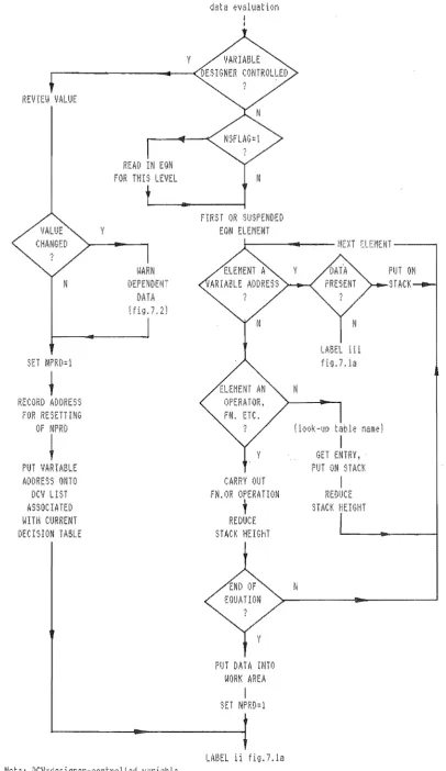
RElJrEI" VALUE

N

SET NPRD=l

t

RECORD ADDRESS FOR RESETTING

OF NPRD

~

PUT VARIABLE ADDRESS ONTO DCV LIST ASSOCIATED WITH CURRENT DECISION TABLE

y

READ IN EON FOR THIS LEVEL

WARN DEPENDENT

DATA

tie;!, 7,2) y

Note: DCIJ=designer-controlled variable

Figu,'e 7. Ib

N

FIRST OR SUSPENDED EON EW1ENT

y

CARRY OUT FN, OR OPERATION

t

REDUCE STACK HEIGhT

PIJT DATA INTO WORK AREA

I

NPRD::1

LABEL ii 7.1a

LABEL iii

f 7,

GET

PUT ON STACK

I

REDUCE

SHCI( HEIGHT

Processing of data

y

FIRST CONDITION

LABEL Ii

fig.7,la

F igLlre 7. lc

decision table execution

NVFLAG=O

I

FIRST Dev ON LIST

Decision table execution

of figure 7.1 a as indicated. The basic principle of recursive descent and the rule scanning process as used by Goel and Fenves (1971) were employed in the T ABEX3 algorithm.

(l) Decision Table Execution

The basis of actual decision table processing, the left-hand path of figure 7.1c, is two nested loops: the outer steps through the rules in a decision table; the inner steps through the conditions in a rule in an attempt to successfully match every condition in a rule to the state of the condition stub.

If a condition entry is immaterial (-), the matching attempt is

omitted and the matching process moves to the next entry in the rule. If

a mismatch Is found the rule is rejected without processing any further entries and processing restarts with the first condition of the next rule. If execution leaves the condition loop normally (through matching the rule with the state of the condition expression), the appropriate rule has been found. If execution leaves the rule loop normally (through there being no matching rule), an error condition exists; this might arise if the table represents an incomplete specification or if data values exceed intended bounds.

expressed in a decision table. An organised arrangement of conditions

and rules can increase decision table processing speed. Possible

ordering tactics are discussed by Humby (1973). In the present project

the arrangement of rules and conditions is entirely the prerogative of

the designer.

57

The TABEX3 algorithm uses a flag (NSFLAG) to indicate whether the

current table is being encountered for the first time. Before processing

of the new table starts the designer is presented with the value of each

of the the designer-controlled variables on the list associated with the

table and is given the option of retaining the current value or entering

a new value (right side of figure 7.Ic). If the value of a

designer-controlled variable alters, all the data in its global

dependence (which will probably include decision table condition

expressions) is set to void and will be recalculated later, if required.

If a designer-controlled variable has "been queried its data presence

flag (NPRD) is set to I (valid) so that it will not be queried again

when other tables are processed during the design iteration. The

addresses of all queried variables are added to the reset list to be

reset to void (NPRD

=

designer the option of changing the value of a listed variable, a check

is made to determine whether the variable is still under the direct

control of the designer. A change in status from being

designer-controlled results if the variable has been edited since the

table with which the list is associated was last run. When a change is

noted, the address of the variable 1s removed from the list.

execution of the table, so that any dependent data is invalidated before an attempt is made to access that data during decision table processing.

(2) Data Evaluation

Before attempting to calculate a variable whose value

undefined a check is made to ascertain whether the variable is under the direct control of the designer; if this is the case the left-hand path of figure 7.1 b is followed. After the designer has been given the

opportunity to change the value of the variable, its storage address is added to the designer-controlled variable list associated with the current decision table. Once on the list, future querying of the value of the variable will be performed before execution of the table begins. All designer-controlled variable lists are built up in this way.

The ri