Existence theorems for floorplans

FOR FLOORPLANS

A Thesis

presented for the degree of

Doctor of Philosophy at the

University of Canterbury Christchurch

New Zealand

by I. Rinsma

LIBRARY

THESIS

mNTENTS

ACKNOWLEDGEMENTS ABSTRACT

I INTRODUCTION

1.

Problems to be studied 2. Organisation of thesis II REVIEW OF THE LITERATURE

1.

Preliminary definitions and explanatory remarks 2. Review of previous work

I I I MAXIMAL OliTERPLANAR GRAPHS AND TREES

1.

Outerplanar and maximal outerplanar graphs 2. Branching index of trees

3. Spanning trees of maximal outerplanar graphs 1V PROPER RECTANGULAR FLOORPLANS

PAGE (i) (iii) 1 2 2 4 4 10 31 31 36 42 67

1. Defining the problems 67

2. Adjacency graphs of proper rectangular floorplans 68

3. Area constraints 70

4. Transforming a graph into a proper rectangular

floorplan 73

5. Counter example for problem B 79

6. Further results 82

v

ISOMETRIC AND ffiNVEX FLOORPLANS 95

1. Isometric floorplans 95

2. Convex floorplans 102

VI

TREE ADJACENCY AND AREA REQUIREMENTS 104

1. Parabolic polygons 104

1. Rectangular floorplans

2. Isometric floorplans

3. Convex floorplans

VI I I SUMMARY. alNCLUSIONS AND FURTHER RFSEARCll REFERENCFS

121

126

131

132

Aa<:NOWLEDGEMENTS

Many people have contributed either directly or indirectly towards the production of this thesis. My main debt of gratitude is to my supervisor, Dr David Robinson, who introduced me to the topic. Without his continuing enthusiasm, guidance and constructive criticism this thesis would never have been completed. Special thanks also go to Dr Derrick Breach who was my acting supervisor whilst Dr Robinson was on leave. I am also very grateful to Dr Brendan McKay and Dr Nick Wormald for their helpful suggestions regarding the proof of theorem 6.4, and Dr John

Hannah

for his assistance in proof reading. Gill Evans is also

to be thanked for her excellent typing.

Finally I wish to thank the Mathematics Department of the University of Canterbury and the University Grants Committee who provided

ABSTRACf

The existence of floorplans with given areas and adjacencies for the rooms cannot always be guaranteed. Rectangular, isometric and convex floorplans are considered. For each, the areas of the rooms and a graph representing the required internal adjacencies between the rooms is given. This thesis gives existence theor.em·s for a floorplan satisfying these conditions. If the graph is maximal outerplanar, only a convex floorplan can always be guaranteed. Floorplans of each type can be four1d if the graph is a tree.

A branching index is defined for a tree, and used to give the minimum number of vertices of degree 2 in any maximal outerplanar graph,

in which the tree can be embedded.

If the graph of adjacencies is a tree, and each room in the plan is external, once again only convex floorplans can always be guaranteed. Rectangular floorplans can always be found in some cases, depending on

aiAPTER I

INTRODUCfiON

An area of research common to architectural design and facility layouts is the designing of planar floorplans, composed of nonoverlapping rooms divided from each other by walls, to suit given topological and dimensional constraints.

Topological constraints are usually adjacencies between rooms and with the exterior of the plan. Interconnections between rooms and with the exterior, and natural lighting or ventilation into the rooms, are often reasons for such constraints. Dimensional constraints involve shapes or sizes of each room and the actual floorplan - for example, rectangular or convex rooms with certain areas, proportions, or lengths of walls.

These constraints interact limiting the choice of feasible solutions. If a plan is to correspond to a rectangular dissection, say, then there are certain limitations on the number and type of adjacencies the overall plan can have. Further, even if a number of solutions exist, they may be difficult to find due to the combinatorial nature of the problem.

The use of computers for automated floorplan design using either heuristics or exhaustive methods is outlined in chapter II.

theoretic approaches have been used over the past twenty years. concentration has been on rectangular floorplans.

Graph Most

point in the investigation, it was unknown whether or not a rectangular floorplan could always be found to satisfy both given adjacency and area requirements.

This thesis studies this problem. The emphasis is on existence theorems. A graph theoretic approach is used.

I.

PROBLEMS TO BE STUDIED

We concentrate mainly on plans in which each room is adjacent to the exterior, and on three types of floorplans. These are defined as rectangular, isometric and convex. The adjacency requirements are represented in a graph. I f each room is external, the graph must be outerplanar (Lynes (1977)), and the allowable graphs range from trees to maximal outerplanar graphs.

For each type of plan we investigate whether a plan can be found to satisfy the areas and adjacency requirements represented either by a tree or maximal outerplanar graph.

II. ORGANISATION OF THESIS

In chapter II preliminary definitions and explanations are given, along with a review of the current literature.

Chapter III is solely graph theoretic. Properties of trees and outerplanar graphs are given. A new index is defined for a tree. This is used to give restrictions on the types of maximal outerplanar graphs any given tree can be embedded in.

graph. These are then extended to the isometric and convex floorplans in chapter V. In chapters VI and VII the adjacency constraints are instead given by a tree. It is shown that at least one floorplan of each of the three types can then be found to satisfy any given area constraints. This is seen not to be the case in chapter VII if the further condition

that each room is adjacent to the exterior is imposed.

OIAPTER II

REVIEW OF THE LITERATIJRE

This chapter reviews the work that has been done on designing floorplans, and the various techniques used to represent the plans. First some preliminary definitions and comments are given. Unless otherwise stated the terminology and notation of Harary (1969) in relation to graphs is used.

I.

PRELIMINARY DEFINITIONS AND EXPLANATORY REMARKS

Definition 2.1 A floorplan is a polygon, the pLan boundary, divided by straight lines into component polygons called the rooms. The edges forming the perimeter of each room are called waLLs.

enclosed by the boundary is called the exterior.

The region not

Definition 2.2 A point in a f loorplan where three or more walls coincide is called a joint. Joints are further classified as n-joints where n is the number of walls that meet at that point.

Definition 2.3 A continuous length of wall between two joints is called a waLL secti.on. This can be either an externaL waLl sect ion, forming part of the plan boundary or an internaL waLL section.

To each floorplan there corresponds a number of graphs.

Definition 2.4 Let every joint in the plan be represented by a vertex, and let an edge exist between two vertices whenever a section of wall in

Definition 2.5 Two rooms in the floorplan are adjacent if they share some wall section. It is not sufficient for them to touch at a point only. Similarly a room is adjacent to the exterior i f it has a wall section in common with the plan boundary.

Definition 2. 6 To each f loorplan corresponds an adjacency graph in which the vertices represent the rooms, and the exterior, and two vertices are joined by an edge whenever there is a wall section in the plan common to both the corresponding regions.

Figure 2.1 shows three different floorplans (a), each with the same plan graph (b) and adjacency graph (c). In each B,E,H,K,L, and M are joints. In (a)(i) room a has walls IK, KH and HI, while the wall sections in the floorplan are KAB, BCDE, EFGH, HIK, HL, LK, LM, BM and EM.

The plan graph is a diagrammatic version of the floorplan. For example, i f in figure 2.1(b) we imagine the edges of the plan to be elastic bands, then it can be "stretched" to form any one of the floorplans in figure 2.l(a).

The plan graph and adjacency graph have a special relationship to each other - the adjacency graph is the dual of the plan graph and viceversa. That is, for each vertex in one graph there corresponds a

face in the other.

From the way in which the plan graph was defined, it follows that the plan graph is always plane. A plane graph has a plane dual, so a graph must be planar if it is to be the adjacency graph of some plan. Also every adjacency graph is connected.

Either the adjacency graph or plan graph or both can have multiple edges. That is, they are multigraphs.

0

G----~

( i)

F

A

c

J

K

B

c

b

J

0

a

L

M

d

c

H

E

0

(iii)

(a)

K

B

L

M

(b) (c)

which is a multigraph. Figure 2.3 shows a plan (a) for which both the plan graph (b) and adjacency graph (c) are multigraphs. ·

A,---Br--_T-C ---;0

F

H

G

F

E

(a) (b)

Figure 2.2 A floorplan (a) and its plan graph (b) .

e

(a)

a

(b) (c)

Figure 2.3 A floorplan (a) whose plan graph (b) and adjacency graph (c) are multigraphs.

Room b in figure 2.3(a) is a through room. Through rooms imply the presence of multiple edges in the adjacency graph.

Definition 2.8 An external room has at least one of its walls forming part of the plan boundary, while an internal room has none.

Definition 2.9 Another type of adjacency graph is called the weak dual by Earl and March (1979). This is the adjacency graph formed as in definition 2.5 above, with the exterior ignored, so each edge represents an adjacency between two rooms in the plan.

Definition 2.10 A rectangular floorplan is a floorplan in which the plan boundary and each room are rectangles.

A. Rectangular floorplans

The following definitions and remarks concern only rectangular floorplans.

Definition 2. 11 Through rooms and corner rooms have exactly two walls forming part of the plan boundary. For corner rooms these walls are adjacent, while for through rooms they are opposite each other.

Definition 2.12 An endroom has three walls on the plan boundary.

Definition 2.13 A wall segment is a maximum continuous sequence of aligned straight wall sections. If each wall section is internal

(external), then it is an internal (external) wall segment.

Definition 2. 14 A fault line is an internal wall segment, joining points in opposite sides of the plan boundary.

and D are corner rooms. All joints in the plan are 3-joints except a which is a 4-joint. The wall segment from

X

to

Y

is a fault line. Rooms E and F are adjacent, but not rooms E and H as they meet only at a 4-joint. Figure 2.4{b) shows that the plan has seventeen internal wall sections and nine external wall sections. Clearly any rectangular floorplan has four external wall segments - the sides of the plan boundary.

Definition 2.15 The four external wall segments of the plan are called the north, south, east and west sides (see figure 2.5).

X

I_

c

A

E

F

B

_{___;_}

a

G

H

0

y

(a) (b)

Figure 2.4 A rectangular floorplan (a) with its wall sections (b).

North

N

West

East

South

Definition 2.16 A north room is a room having a wall on the north side. Similar definitions exist for south, east and west rooms. A corner room, like C in figure 2. 4 is therefore both a north and east room.

Definition 2.17 For a given floorplan, let the sets V and H consist of those internal wall sections which are parallel to the west or north sides of the plan respectively. Then {V,H} is a partition of the set of

internal wall sections in the plan.

Definition 2.18 The floorplan with one room is called trivial, and generally will be excluded from the discussion.

B. Properties of rectangular floorplans

The following need no proof.

1. Every rectangular floorplan has at most two endrooms. 2. Every rectangular floorplan has at most four corner rooms. 3. Since walls meet at right angles, only 3-joints and 4-joints

are possible in any rectangular floorplan.

II.

REVIEW OF PREVIOUS WORK

The remainder of this chapter outlines the research made into the design of floorplans, particularly rectangular, with given topological or dimensional constraints.

given.

A. Representing rectangular floorplans

1. Gratings

Mitchell, Steadman and Liggett (1976) introduced minimal gratings, arising from the work of Newman (1964) to describe rectangular floorplans. A coordinate system or grid is imposed on the floorplan, with every grid line corresponding to at least one wall in the floorplan, using the minimum number of grid lines possible to mark the position of all walls.

Consider figure 2.6(a) in which two floorplans have essentially the same ' shape' . In (b) the gratings of each floorplan are shown superimposed on the plan. The dimensions of the minimum gratings can be adjusted so that each cell in the grating becomes square, as shown in (c). This representation is unique and is called the dimensionLess representation or canonical version of the plan.

It does not alter the topology of the original figure, as rooms adjacent in the plan remain adjacent in the canonical version. Also it

is possible to return to any original dimensional floorplan from the dimensionless version with an appropriate set of dimensions, giving the required spacings for the grating in the x and y directions.

The grating size of any grating is given by L x m, where m is at least equal to

L.

Thus the grating in figure 2.6 has size 2 x 3.

(a)

•r--

I'

"

\

.r

,

(b)

t;:.

...

,

(c)

Figure 2.6 Two floorplans (a) with their gratings (b) and identical dimensionless representation (c) .

2.

Isomorphic floorplans

Definition 2.19 Let and be two undimensioned labelled rectangular floorplans whose sets of internal wall sections have

i) the rooms in F1 are in one-to-one correspondence

to the rooms in F2 ,

ii) two rooms in F1 are adjacent if and only if the

iii) the internal wall sections in vi are in one-to-one correspondence to those in V2 , and H1 to H2 , or Vi to H2 and Hi

to V2 •

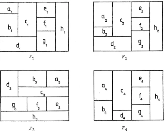
Here part (iii) deals with isomorphisms of floorplans under either rotation of 90°, 180° or 270°, or reflection in a mirror line parallel to one of the sides, or a combination of both.

Three of the four floorplans in figure 2.7, namely Fi,

F2

and F3

are isomorphic. Fi and F4 satisfy (i) and (ii) above but not (iii). Vi corresponds to V2 and H3 , while Hi corresponds to H2 and V3 •

Note that the adjacencies of rooms to the exterior is not used in the definition for isomorphism. This is because, as is sho'rn later, once the plane weak dual and sets V and H of a floorplan are known, the rooms adjacent to the exterior, their type and the order in which they occur around the plan boundary can be found.

Note also that isomorphism is an equivalence relation.

a1

e

₁

e

₂

a

c

~

b1

1

h

1

2

s

b2

~

h2

d

g1

1

d2

g

2

d

~

a3

3

(3

~

a

4

c

4

t

h4

~

~

e

3

h3

~

~

~

Figure 2.7 Four labelled undimensioned rectangular floorplans with the same weak dual. ,

F

3. Trivalent and fundamental floorplans

Consider the two floorplans (a) and (b) shown in figure 2.8.

(a) (b)

If'

'

,

(c)

Figure 2.8 Two floorplans (a) and (b) with the grating (c) of (a) .

In (b) there is a 4-joint while in (a) none exist. The minimal grating corresponding to (a) is shown in (c) where x1 , x2 , x3 , y1 , y2 are

the dimensioning variables. If x2 is set equal to zero, then plan (a) is

transformed into plan (b). That is the two 3-joints collapse into a single 4-joint, as shown in figure 2.9.

Floorplans in which all joints are 3-joints have been called trivaLent.

Another problem with gratings can also occur. Consider the two floorplans shown in figure 2.10{a), and the corresponding gratings in {b). In { ii) two of the internal wall sections are aligned and hence correspond to the same grid line, while in (i) they do not. If y₂ is set equal to zero in {i) then the grating shown on the right is obtained. Thus the 'aligned' floorplan can be treated as a particular type of

'nonaligned floorplan'.

A nonaligned floorplan which is also trivalent has been termed fw-tdamenta"L.

( i) (ii)

(a)

,

..

;~

'

....

,

,

(b)

B. Generating and counting rectangular floorplans

A rectangular floorplan can be thought of as either the addition of rectangular pieces, like tiles, to produce a rectangular plan, or the division of a large rectangle into smaller rectangular pieces. The latter case has been called a rectanguLar dissection. Many different approaches have been used to enumerate rectangular floorplans.

The first attempt to devise an algorithm to generate rectangular dissections was made by Steadman (1973) using a dissection method. This was not exhaustive. A second algorithm, by Mitchell et al (1976), used three operations, of both addition and dissection type, applied to all dissections with n-1 rectangles to generate dissections with n rectangles. This was implemented as a computer program by Sauda (1975) and used to generate dissections up to n = 8. However Earl (1977) showed this was not exhaustive for n

=

16. He devised a new algorithm, claiming it to be exhaustive for all n. His method, unlike the earlier ones, produced only fundamental dissections.

Flemming ( 1978) developed a new way of describing plans, called walL representations, a more general approach than gratings, to provide an exhaustive enumeration of trivalent dissections.

Bloch (1976) predicted theoretically the range of grating sizes needed for all dissections with n rectangles. From this a til algorithm was devised:- each feasible grating size for a particular value of n was divided into n rectangular tiles, and then checked to see whether they could be placed together in such a way to fill an empty grating of the predetermined size. From this he was able to generate all dissections upton= 19 (Bloch (1979a, 1979b)).

The exact number of dissections in the various categories, with or without alignments or 4-joints were given by Bloch and Krishnamurti (1978) for values up to n

=

10. These were mainly due to Krishnamurti (Krishnamurti and Roe (1978), Bloch and Krishnamurti (1978)) who designed another method of generating dissections, essentially by assigning imaginary colours to the grating cells. Four rules were given, and the various classes of dissections mentioned above, were generated using different combinations of the rules. A minimum colouring was used to ensure only nonisomorphic rectangular floorplans were produced, making it an extremely fast algorithm.

Another categorisation of rectangular floorplans by Combes (1976) gave properties of a graph relating the number of external walls to internal walls, pa.rti. ti.ons, for each rectangular dissection with n rectangles. He also demonstrated various general relationships existing between the number of external and internal walls, and the number of 3-joints and 4-joints, and n, for a rectangular dissection. These relationships were shown later by Gutierrez (1979) to be derivable from Euler's polyhedral formula, and graph theory.

As will be shown in Section D, graphs have also been used to represent and enumerate floorplans.

An objection by Stiny (1979) to the work so far was that rectangular dissections represented a restricted class of designs.

C. Nonrectangular plans

March, Matela and O'Hare have done similar work on polyominoes. March and Matela {1974) categorised polyominoes in a way similar to Combes, while Matela and O'Hare (1976) investigated some of the relationships between polyominoes and their weak dual adjacency graphs.

can be represented by rectangular floorplans, by subdivision or adding 'dummy' rooms. (Steadman (1983)).

Earl (1980) proposed a classification to include all architectural arrangements whose walls are along one or other of two perpendicular directions. This was based on the nature of endpoints of walls in an arrangement. He showed that many of the graph-theoretic representations of rectangular floorplans, and those forms used by Flemming (1978) and Mitchell et al (1976), were related at a more general level. He used shape grammars, developed by Stiny (1975) and Gips {1975) as a special design language involving Boolean operators and description functions specifying how various two-dimensional and three-dimensional shapes may be assembled together, to construct his classes of shapes.

There are many classes of regular nonrectangular floorplans, for example, plane tessellations in which tiles of one or more different shapes are packed together in repeating patterns to fill the plane (Krishnamurti and Roe (1979)), or triangular and hexagonal analogues of polyominoes (Lunnon (1972)).

However, studies of actual building (Bemis (1936), KrUger (1979)) have shown these types are rather rare. KrUger, for example, studied all the buildings in the city of Reading, and found 98% of them to be of rectangular geometry.

Both Krishnamurti (1979) and Earl (1978) have extended their enumerations to the third dimension, that is, to packing rectangular blocks within a rectangular box.

D. Graphs of floorplans

1. Types of graphs

As mentioned in Section I of this chapter, the floorplan can be described as a pLan graph, in which the vertices are the joints, and the edges wall sections between joints, of the floorplan. This diagrammatic version is similar to the bubble diagrams used by Korf (1977).

The adjacency graph and the weak duaL have vertices representing regions, and edges adjacent regions of the floorplan. The adjacency graph is the dual of the plan graph, unlike the weak dual which is concerned only with internal adjacencies between rooms. Thus there is a vertex in the weak dual for every room in the floorplan, an edge for every internal wall section, and a face for every internal joint.

As the plan graph is planar, every adjacency graph and weak dual is planar. Furthermore the two types of adjacency graphs are connected. If the rectangular floorplan has no through rooms, the adjacency graph has no multiple edges or loops, and the weak dual has no cut vertices.

Adjacency relationships are important, for whenever two rooms share a sufficient length of wall, then it is possible for them to be made accessible to each other via a door. Also overall patterns of adjacency determine circulation routes for a building. Further, rooms having adjacencies to the exterior can have windows thus providing natural lighting, and ventilation.

In fact, Levin (1964) and Hillier and Hanson (1984) used an access graph in which the vertices represented the rooms or exterior of a

floorplan, and each edge the existence of a door or means of access between two regions.

corners of the floorplan. Adjacencies of rooms to these regions and the adjacencies between the four regions themselves were added to the weak dual.

Figure 2.11 shows a rectangular floorplan (a) with its plan graph (b), adjacency graph (c), weak dual (d) and augmented dual (e). Rooms b and d are not adjacent as they meet only in a point.

2. Colouring an adjacency graph

Many floorplans can have the same weak dual, as is shown by figure 2.12.

The edges of any adjacency graph or weak dual of any rectangular floorplan can be coloured in either of two 'colours • to specify the directions in which the corresponding walls lie. Reflecting a given rectangular floorplan in a line parallel to one or other of the sides of the plan, or rotating it 180° or 360° does not alter the directions in which the walls lie. However, rotating it 90° or 270° makes all north-south walls lie east-west and viceversa. Thus two labelled rectangular floorplans F1 and F2 are isomorphic if either their

corresponding coloured adjacency graphs (or weak duals) are identical, or each edge in the coloured adjacency graph (or weak dual) of plan F1 is

coloured differently from the corresponding coloured edge in the adjacency graph (or weak dual) of plan F2 .

This colouring must obey specific rules, if the corresponding plan is a rectangular floorplan (Grason (1968), Earl and March (1979)).

a

b

c

d

e

f

(a) (b)

(c) (d)

(e)

2.11 The various graphs associated with floorplans:-plan graph (b), adjacency graph (c), weak dual (d) and

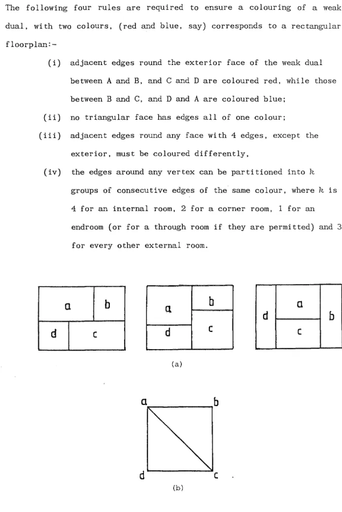
The following four rules are required to ensure a colouring of a weak dual, with two colours, (red and blue, say) corresponds to a rectangular

floorplan:-(i) adjacent edges round the exterior face of the weak dual between A and B, and C and D are coloured red, while those between B and C, and D and A are coloured blue;

(ii) no triangular face has edges all of one colour;

(iii) adjacent edges round any face with 4 edges, except the exterior, must be coloured differently,

(iv) the edges around any vertex can be partitioned into k groups of consecutive edges of the same colour, where k is 4 for an internal room, 2 for a corner room, 1 for an

endroom (or for a through room if they are permitted) and 3 for every other external room.

a

b

b

a

d

b

d

c

d

c

c

(a)

(b)

Figure 2.13 gives an example of a floorplan and its corresponding coloured weak dual. Here a corresponds to an endroom, while d and t are corner rooms. All of a's incident edges are red, while d has edges of both colours, arranged red, red, blue in cyclic order around d.

Note that the blue and red edges correspond to the sets V and H of the floorplan (recall definition 2.17). The rules arise from the properties of rectangular floorplans - namely at any 3-joint, two wall sections run in one direction, and the third in the perpendicular direction, and each room has four walls, two in each direction.

b

c

f

d

e

a

a

h

g

_I

(a) (b)

Figure 2.13 Colouring of the weak dual (b) corresponding to floorplan (a) .

3. Primary plans

A planar graph to which no edges can be added without making it nonplanar is maximal pLanar. Every face in a maximal planar graph is a

4.

Graph representations of a dimensioned rectangular floorplan Both the augmented dual graph and a type of 'electrical' graph can be used to represent the dimensions of a rectangular floorplan. A coloured augmented dual with adjacencies between the exterior regions omitted, can be split into two subgraphs or 'half-graphs' (Mitchell et al, (1976)) corresponding to the two colours.

The vertices in each 'half-graph' represent the rooms and two exterior regions of the plan. Each edge represents a wall section in the plan, and can be weighted by the length of the corresponding wall section. Further each edge can be assigned a direction, so that all edges in each 'half-graph' are directed the same way, say west-east, to form a network. Then the total weight of edges leaving the source, say west, equals the total weight entering the sink, east, and is the overall dimension of the plan from north to south. Further, the total weight of edges entering every other vertex in the 'half-graph' equals the total weight of edges leaving the vertex. This condition corresponds to one of Kirchhoff's two laws for current in an electrical network (see figure 2.14).

Another type of network, introduced by Brooks, Smith, Stone and Tutte (1940) when 'squaring the square', having properties parallel both of Kirchoff's laws was used by Teague (1970) and March and Steadman

(1971). Vertices now represent each maximal continuous straight run of wall running west-east (or north-south), that is, each wall segment. A pair of networks exists for each plan, the sources being the west (or north) sides and the sinks the east (and south) sides of the plan. The edges represent the rooms of the plan. Each vertex is given a value

Either one of the two networks completely represents the dimensioned plan. See figure 2.15 for the west-east network corresponding to the floorplan in figure 2.14.

8 5

a

6

b

8

2

c

d

e

4

4 4 5

(a)

12 1 2

w

E

5

(b)

Figure 2.14 The two half-graphs (b) of floorplan (a).

8 5

a

a

6

"'

b

6

8

2

c

{3

d

e

4

12 12 6 9 6 5 4 0 12

4 4 5

(a) (b)

The two networks contain the same number of edges (rooms) and if the edges entering the sink and leaving the source are omitted, they are duals.

Roth, Hashimshony and Wachman ( 1982) also used this type of representation but with the weights of the edges representing distances between the walls. Stockmeyer (1983) and Otten (1982a, 1982b) also used similar representations.

E. Designing floorplans

So far we have reviewed ways of counting and representing rectangular plans. We turn now to questions of design in architectural practice and facility layouts - that of finding floorplans that satisfy given constraints.

Usually all the rooms are specified, and some adjacency requirements between rooms, and the exterior. These can be shown in an adjacency requirement graph, where vertices represent the rooms, and exterior, and edges the required adjacencies. When a floorplan is drawn, other adjacencies not specified may occur. Thus the adjacency requirement graph will be a spanning subgraph of the adjacency graph of the final plan. There is the possibility that the adjacency requirement graph is nonplanar in which case not every requirement can be satisfied. The problem is to realise the given adjacency graph as a rectangular floorplan. As seen earlier there could be many different floorplans corresponding to the given graph. Also the graph might have more than one embedding in the plane. Further there may be constraints on dimensions and areas of rooms, limiting the choice of floorplans.

Levin (1964) was the first to apply graph theory to architectural design. Concentrating on access graphs of graphs, he enumerated all outerplanar graphs and their possible labellings up to n

=

4. He also showed that certain access graphs (namely K5 ) cannot be realised in

floorplans; that is, no floorplan has K6 as its access adjacency graph. The second half of his paper de~lt with a heuristic method to find an optimal access graph and plan based on cirulation criteria.

Cousin (1970) and Friedman (1975), followed Levin's lead, by looking further at graph-theoretic ideas. The study of floorplans also arose in facility layouts, a branch of operations research. Many authors, for example, Krejbi'fik (1969), Seppanen and Moore (1970), Hashimshony, Shaviv and Wachman ( 1980) were concerned with the problem

that the adjacency requirement graph was not planar. They examined tests of planarity, and methods of selecting that minimum 'resolving' set of edges which removed from the adjacency requirement graph changed it into a planar one.

This work was criticized by Steadman (1983) as being unrealistic, for nearly always in architectural practice the adjacency requirement graph is planar.

minutes, for example, to produce all five solutions to a five-room problem. Grason himself said that for more than eight rooms, a heuristic search technique would need to be developed.

the dimensions were given as fixed values.

Another problem was that

Gilleard (1978) outlined a related method under development. The question of 'well-formedness' was looked at by Earl and March (1979).

Here they gave the necessary and sufficient conditions for any graph to be the augmented dual or weak dual of a rectangular floorplan without 4-joints. Further they showed that every colouring of such a graph satisfying the colouring rules given earlier, once corners are chosen, produces an oriented floorplan.

A different approach was developed by Mitchell et al (1976) based on the work by Steadman (1973). The first stage found all dimensionless rectangular dissections satisfying the required adjacencies. This was done by searching through a given catalogue of topologically different dissections, with up to eight rectangles (the catalogue mentioned earlier). Dimensions were satisfied by solving a set of simultaneous linear equations which specified lengths, widths or proportions of individual rooms. This was done using either linear programming minimizing or maximizing overall plan length, width. perimeter or proportion. Area requirements require quadratic equations and were solved using nonlinear programming.

Gero (1977) suggested dynamic programming gave better results for the dimensioning stage. However the main disadvantage of this approach was its dependence on the catalogue of rectangular dissections, which as discussed earlier has only been enumerated up to ten rectangles.

all solutions where constraints were reasonably tight for small number of rooms (Steadman (1983)).

Galle (1981) following the approach of Mitchell et al (1976)developed an exhaustive floorplan generating algorithm for rectangular plans on modular grids which minimized the number of cells in the smallest room. Test results showed realistic problems of up to ten rooms solved in modest computer time.

Baybars (1982) outlined a graph-theoretic technique for the generation of plans without circulation spaces, using an operation called 'wheel expansion' to generate the maximal planar underlying graphs. This operation was outlined in an earlier paper (Baybars and Eastman (1980)) but was later cri tized by Earl (1981) as being the dual of the face splitting operation of March and Earl (1977) used in ornamentation.

The most recent work similar to Grason is that of Roth et al {1982). Starting from the adjacency requirement graph, non-required adjacencies were added, and the graph split into two subgraphs. These were then converted into networks, vertices representing parallel walls and edges the distance between them, or the dimensions of the rooms. Using the PERT technique for finding the critical path, all edges on the critical path were given their minimal dimension. Combinations of other dimensions were then determined to find a feasible realization. The method appeared successful with as many as twenty rooms, and has been modified to include non-convex rooms and plan boundary.

Korf (1979) criticized the restriction of existing methods to rectangular floorplans and proposed drawing the duals of embedded adjacency graphs as 'bubble diagrams'. However this neglects the fact that any actual floorplan would eventually have to be realised with definite room shapes and dimensions.

aiAPTER III

MAXIMAL OUI'ERPLANAR GRAPHS AND TREES

This chapter reviews and introduces the graph theory necessary for the remainder of the thesis. The first section describes outerplanar and maximal outerplanar graphs. In section II, a new index ~ for trees is introduced, and its properties investigated. The remainder of the chapter concerns the embedding of a tree in a maximal outerplanar graph G, and the relationship between ~ and the number of vertices of degree 2

in G.

Throughout, the notation and terminology of Harary (1969) is used, unless stated otherwise. In particular, all graphs are finite, loopless, connected and without multiple edges.

I . OUTERPLANAR AND MAXIMAL OUTERPLANAR GRAPHS

Outerplanar and maximal outerplanar graphs have often occurred in the recent literature.

without proof .

This section details their properties, mainly

Definition 3.1 A planar graph is outerpLanar if it can be embedded in the plane so that every vertex lies on the exterior face.

Theorem 3.1 [Harary (1969)] A graph G is outerplanar if and only if each of its blocks is outerplanar.

Theorem 3.3 [Colbourn and Booth {1981) or Syslo (1979)] Every 2-connected outerplanar graph having at least three vertices possesses a unique hamiltonian cycle.

Corollary 3.4 Every vertex of a 2-connected outerplanar graph has degree at least 2.

Corollary 3.5 [Mitchell (1979)] Every 2-connected outerplanar graph with n vertices is isomorphic to an n-gon divided into polygons by chords.

Definition 3.2 An outerplanar graph G with n vertices is maximal outerpLanar if no edge can be added toG without losing outerplanarity.

Theorem 3.6 [Harary (1969)] Every interior face of a maximal outerplanar graph is a triangle.

Theorem 3.7 [Harary (1969)] Every maximal outerplanar graph with n vertices is a triangulation of some polygon P with n points.

n

Theorem 3.8 [Harary (1969)] Let G be a maximal outerplanar graph with n ;:: 3 vertices.

Then G has

(i) 2n-3 edges

(ii) n-2 interior faces

(iii) at least two vertices of degree 2

(iv) at least three vertices of degree not exceeding 3.

Theorem 3.9 [Mitchell (1979)] Let G be a maximal outerplanar graph with n ;:: 3 vertices. Then G does not have a vertex u of degree 2, whose

Corollary 3. 10 A maximal outerplanar graph G with more than three vertices does not have two vertices of degree 2 adjacent.

Proof: (By contradiction). Assume u and v are adjacent vertices of

degree 2 in G. Let their other neighbouring vertices be w and x respectively, with

w

~

x.

Then from theorem 3.9

v

and

w

are adjacent so that v has degree at least 3, contradicting the original assumption. #

More important is the following well known result concerning the recursive construction of any maximal outerplanar graph. (See Proskurowski {1979), for example.)

Theorem 3.11 A graph is maximal outerplanar if and only if it can be constructed from a triangle (K3 ) by a finite number of applications of

the f o 11 owing procedure : to the graph already constructed add a new vertex u in the exterior face and join it to two vertices v and w

adjacent in the exterior face.

manner

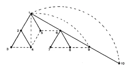
Figure 3.1 shows a maximal outerplanar graph constructed in this from the initial triangle labelled 1,2,3. The t th vertex for t

L

3 is joined to two vertices having labels less than t.

Definition 3.3 From a graph G, the subgraph G - u is formed by deleting vertex u and all edges incident with u.

12

Theorem 3.12 [Mitchell (1979)] If G is a maximal outerplanar graph with n

>

3 vertices, then for any vertex u with degree 2 in G, G- u is maximal outerplanar.

Lemma 3.13 Let G be a maximal outerplanar graph with hamiltonian circuit

C.

For every two distinct vertices rands in

G,

there exist two distinct paths consisting entirely of edges in C from r to s; one going clockwise from r to s around the circuit, the other anticloc~rise.

Theorem 3.14 Let G be a maximal outerplanar graph with hamiltonian circuit

C.

Let r,s,t,u be distinct vertices in

G

with r joined to s by an edge not in C, and t joined to u by an edge not in C. Then both t and u are in the same path consisting entirely of edges in C from r to s. Proof: If t and u are in different paths consisting entirely of edges in C, we have the situation shown in figure 3.2. The edges {r,s} and {t,u} intersect at a point within the hamiltonian circuit which is a contradiction, since

G

is maximal outerplanar. #

Figure 3.2 The situation for theorem 3.14.

Theorem 3. 15 Let G be a maximal outerplanar graph with hamiltonian circuit C, and let r and s be two distinct vertices joined by an edge not in C. Further let w

1,w2, ... wi be the vertices in order as they occur in one of the paths consisting of edges only in C from r to s. Then the subgraph H of G induced by the vertices w

1, w2, ... wi, r, s is maximal

outerplanar and at least one

w

Proof: The subgraph H has a hamiltonian circuit passing through the vertices r, w

1,w2, ... wt,s in order, and hence is outerplanar. Now. _J is adjacent in G to a vertex u that is in G but not in H, for then they would be joined by an edge not in C and would be in different paths consisting entirely of edges in C from r and s, contradicting theorem 3.14. Each w. is therefore adjacent to the same vertices in Has in G.

J

As G is maximal outerplanar, by theorem 3.6, each interior face in G is a triangle. Thus each interior face in H is also a triangle, and H is maximal outerplanar.

Vertices r and s do not have the same degree in H as in G, but since they are adjacent in H, by corollary 3.10, at most one of them has degree 2 in

H.

By theorem 3.8,

H

must have at least one vertex other than r or s with degree 2. Thus at least one

w.

has degree 2 in H, and

J so also has degree 2 in G.

A. Enumerating maximal outerplanar graphs

Beineke and Pippert {1972) showed that the number of nonisomorphic maximal outerplanar graphs with n vertices,

IG

1.

where n

>

3 is given by

n

IG I

_n = _{2n t(n-2) +} 1

2

1 t ( 2 ) n-3 + ~ ₄ t(n-2) + ₂

l

₃ (n-3) ₃ where t(x) = { (2x)! if x integer

x~ (x+1)!

otherwise.

Table 3.1. The number of nonisomorphic maximal outerplanar graphs

jG j,

n

divided into groups according to the number of vertices with degree 2.

Number of vertices Number of vertices of degree 2 Total number of graphs

n 2 3 4 )4

IG I

n

3 1 1

4 1 1

5 1 1

6 2 1 3

7 3 1 4

8 6 5 1 12

9 10 14 3 27

10 20 42 19 1 82

11 36 112 73 7 228

12 72 304 295 62 733

II

BRANCHING INDEX OF TREES

Definition 3.4 A tree with n vertices in which every vertex has degree

1 or 2 is called a path graph

P.

n An isolated point is considered as

A path graph P with one vertex being a root, is called a rooted

n

path graph. A tree is branching if it is not a path graph.

Definition 3.5 Given a tree T with root u, delete the root. What is

left is a collection of k. subtrees, where k. is the degree of u. Each

subtree is taken as rooted at the vertex that was initially adjacent to

u. The number of these rooted subtrees which are branching is called the

branching index of u, and denoted by ~(u) or ~- The branching index for

each vertex of an unrooted tree is obtained by treating each vertex in

Lemma 3.16 Let u be a vertex in tree

T

with ~(u)

l

2.

If w "/. u is another vertex in T, then the subtree of T-w which contains u is branching.

Proof: Since ~(u)

l

2 and w is one of the subtrees of T-u, there are at least ~(u)-1 subtrees of T-u which are branching and do not contain

w.

These are included in the subtree of T-w containing u. follows.

The result

Lemma 3.17 Let u be a vertex in tree T with one of the subtrees in T-u being a path graph. Let Z be this subtree. Then every vertex w in Z has branching index at most 1 in

T.

Proof: For each

w

in Z, all the subtrees of

T-w

not containing u are subtrees of Z and hence are path graphs. Thus only the subtree of

T-w

containing u can be branching. The result follows.

Theorem 3.18 In any tree

T

the vertices with ~

l

2 induce a subtree, or there are no such vertices.

Proof: Let

B

be the set of vertices with ~

l

2. If

B

is not empty, assume the subgraph of T induced by the vertices in B is not connected. Then there exist two vertices u and v in B which are not adjacent in T, and another vertex w not in B, which is on the path joining u to v in T. Thus u and v are in different subtrees of

T-w.

Since ~(u)

L

2, by lemma 3.16 the subtree of T-w containing u is branching. Similarly the subtree of T-w containing v is branching. Hence

T-w

contains at least two branching subtrees, implying w€B which contradicts the original assumption. Thus the subgraph of T induced by B is connected and is a

tree. #

Proof: If no vertices have~= 2, the result follows. However if there are vertices in

T

having ~

=

2, assume the subtree S induced by them is not a path graph. Then there exist distinct vertices w, x, y, z in S, where w is on the path in S between x and y, but z is not, and each of w,x,y,z has ~

=

2.

The situation is as shown in figure 3.3.

X

Figure 3.3 The situation in theorem 3.19.

Since ~(y)

=

2, by lemma 3.16, the subtree of

T-w

containing y is branching. Similarly, the subtree of

T-w

containing z, and that containing x are branching. Thus

Mw)

l

3 which contradicts the original

assumption. #

Remarks: All vertices in a tree can have branching index of 0. This only occurs i f the tree is itself a path graph or is that shown in figure 3.4.

Trees with all vertices having ~

=

0 or 1 only also exist. Some examples of these are shown in figure

3.5.

Each vertex has its branching index written alongside.

0

Figure 3. 5 Trees in which each vertex has [3 = 0 or 1 .

Lemma 3.20 A tree with vertex u having ~{u)

=

0 cannot have any vertex v with ~(v) ~

2.

Proof: From lemma 3.16. #

Definition 3.6 The Linking subtree of a tree T induced by vertices in the set V ={a, b, c, ... , r} is the subtree ofT induced by Vandall vertices u in T but not in V lying on a path in T between any two distinct elements of V. It is thus the minimum subtree of

T

containing set V.

Definition 3.7 For any vertex x in a tree T, de~{x) denotes the degree of x in

T.

Theorem 3.21 Let T be a branching tree, and let D be the linking subtree of

T

induced by vertices x with de~(x) ~ 3. Every vertex in

T

has branching index of 0 or 1 if and only if

either {i) exactly one vertex x in T has de~(x) ~ 3,

Proof: We first prove the sufficiency.

{i) If exactly one vertex x has de~(x) ~ 3, each of the subtrees in

T-x

is a path graph. Thus ~(x) = 0, and every other vertex

v

in

T

has ~(v) ~ 1 by lemma 3.17.

(ii) Assume at least two vertices in

T

have degree at least 3 and let D be the linking subtree induced by them. Let the diameter of D be d.

If d = 1, then

D

consists of two vertices u, u joined by an edge. Every other vertex in T has degree 1 or 2. Thus each subtree of T-u except that containing v is a path graph. Let Z be one of these subtrees. By lemma 3.17, each vertex

w

in Z has ~(w) ~ 1 in

T.

If the subtree of

T-u

containing

u

is branching, ~(u) = 1. Otherwise ~(u)

=

0. Similarly ~(v) ~ 1, and any vertex y in a subtree of

T-v

not containing u, has ~(y) ~ 1. So each vertex x in T has ~(x)

=

0 or 1.

If d=2 and at most one terminal vertex u in D has de~(u)

>

3, then D is as shown in figure 3.6 where ~ ~ 1. From the definition of D, it follows deg,.,.,(w .) = 3 and the subtree of

T-v

containing w. is a path

-1 J J

graph, for every j from 1 to 2. Thus as above, each vertex x in T has

~(x) = 0 or 1.

If d = 3 and no terminal vertex y in

D

has de~(y)

>

3, then

D

is as shown in figure 3.7.

Here k ~ 1 and 2 ~ 1, and de~(zt) = 3 for each t from 1 to k. Also de~(wj)

=

3 for each j from 1 to ~. All vertices in

T

but not in

D

w

u

have degree 1 or 2. Thus each subtree of T-u not containing v is a path graph. Similarly each subtree of

T-v

not containing u is a path graph. Thus from lemma 3.17 and above, each vertex x in

T

has ~(x)

=

0 or 1.

Figure 3.7 A tree with d=3.

To prove the necessity, let T be a branching tree in which each vertex has ~(x) = 0 or 1. Then exactly one vertex !J in T may have

de~(!J)

2

3. Otherwise, assume

D

has diameter d

>

3. Then there exists two terminal vertices in D, u and u, and a path< u,w

1, w2, ... ,wr, v

>

from u to v in D, with r

2

3. The subtree of T-w

2 containing w1, also contains u, and since de~(u) ~ 3 it is branching. Similarly the subtree of T-w

2 containing w3 also contains v and is branching. Thus ~(w

2

)

2

2

which is a contradiction. So d ~ 3.

I f d = 3, D is of the form shown in figure 3. 7. Suppose some terminal vertex z₁ has de~(z

1

)

>

3. As de~(w

1

)

2

3, it follows that both the subtree of T-u containing z

1 and the one containing w1, are branching. Thus ~(u)

2

2, a contradiction.

If d

=

2 and at least two terminal vertices, u and w

1 say, have

degree greater than 3 in

r.

then by a similar argument considering figure 3.6, ~(u)

2

2, which is a contradiction.

If d

=

1, so that

D

consists of two adjacent vertices u, and u, both de~(u)

2

3 and de~(u)

2

3.

III

SPANNING TREES OF MAXIMAL OUTERPLANAR GRAPHS

Lemma 3.22 Every tree with n vertices, where n

>

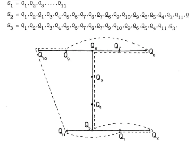
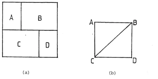
2, can be embedded as a spanning tree of a maximal outerplanar graph with n vertices.

Proof: Given a tree T, select any vertex to be the root. Perform a depth-first search of the vertices starting from the root (Aho, Hopcroft and Ullman (1974)). Number the vertices 1, ... n in increasing order as they are visited. Redraw the tree with the root at the top, and let the neighbours of each vertex x with labels greater than x be drai~ so that they occur in increasing order from left to right across the page. Add edges to T, where necessary, joining each vertex i to vertex i+1 for i ranging from 1 to n-1, and joining vertex n to the root. An outerplanar graph with an hamiltonian circuit passing through the vertices in numerical order results. Adding edges to triangulate each interior face of the graph results in a maximal outerplanar graph G. #

Figure 3.8 shows a tree embedded in a maximal outerplanar graph in the manner outlined by lemma 3.22.

---

---3

Theorem 3.23 [Nebesky {1976)] Let

T

be a spanning tree of a maximal outerplanar graph G with hamiltonian cycle C. If vertices r,s,t,u are such that t and u belong to distinct components of the graph C-r-s, then the path in

T

from r to s, and the path in

T

from t to u have at least one vertex in common.

Theorem 3.24 Any maximal outerplanar graph G with n vertices has a minimum of 2 and a maximum of

vertices of degree 2.

~ if n is even, or 2

Proof: From theorem 3.8 and corollary 3.10.

!::!:_1

2 i f n is odd,

Theorem 3.25 Let T be a spanning tree of a maximal outerplanar graph G

with n ) 3 vertices and hamiltonian cycle C. Let D be the 1 inking subtree of T induced by the vertices having degree 2 in G. This tree consists of m vertices u₁,u₂, . .. ,um ofT. Let the remaining vertices of

T be labelled v

1,v2, ... ,v n-m in order as they occur clockwise around C.

Proof: there

Then {i) if vj is adjacent to vk in T, {v

1

,vk} is an edge inC,

{ii) if vj is adjacent to some ui in T, the subtree of T-ui containing vj is a path graph,

and {iii) ~(vj) ~ 1 in T,

for each j between 1 and n-m.

{i) Assume _{v j ' vk} is an edge not in

c.

Then by theorem 3.15, is a vertex _~ having degree 2 in G, which is in the path consisting entirely of edges in

c

from v. to _vk and going clockwise

J

around the circuit. Similarly, there is a vertex u with degree 2 in G !:1

in the path consisting only of edges in C from v j to vk and going anticlockwise around the circuit. Thus {when G is embedded in the plane), we have the situation shown in figure 3.9.

Vertices ux and u!J belong to different components of C-v

1-vk' and

from u to u have at least one vertex in common. Since the path from v.

X y J

to vk in T is the edge {vj,vk}' the vertex common to both paths is either vj or vk. But, from the definition of D, each vertex in the path from ux

to u is labelled some u.. Thus we have a contradiction.

y ~

V.

J

Figure 3.9 The situation in theorem 3.25.

(ii) In T, vj can be adjacent to at most one of {u

1,u2, ... um} or else there is a circuit. Because of the way in which the vertices were labelled and (i) above, only v.

1( ..J ) ' or

J- mou. m v. 1 ( ..J ) ' or both

J+ mou. m

can be neighbours of vj in

T

provided _{{vj,vj-1(mod. m)} or} {v .. v.

1( ..J ) } respectively are edges in C. J J+ mou. m

The possibilities for v. in T, taking subscripts modulo m, J

therefore are:-(1)

(2) (3) (4)

degree 1, adjacent only to some

u.;

~

degree 2, _{adjacent to u. and one of vj_}

1 or vj+ 1 ; ~

degree 3, adjacent to u. and both v.

1 and v j+1;

~

J-degree 1, not adjacent to any u .• adjacent to v. 1

~

J-(or vj+1);

(5) degree 2, not adjacent tout, adjacent to both vj_ 1 and vj+1'

If v. is adjacent to u., the subtree (which may be quite long) of

J ~

T-ut containing v j cannot contain any other vertex u.e, or vertex v _s

subtree of

T-u.

containing u. must therefore be a path graph.

L J

(iii) If u. is not adjacent in T to some u., then since T is

J L

connected, there is a path in

T

from uj to some uk with ~R adjacent in

T

to some u .

r The subtree of T-ur containing uk also contains uj and by (ii) above is a path graph. Hence by lemma 3.17, {3(uj) ~ 1. Also by lemma 3.17 and (ii) above, if uj is adjacent to some ut' {3(vj) ~ 1.

Thus all three cases of the theorem hold.

A given tree

T

with n vertices can be embedded as a spanning tree of two maximal outerplanar graphs

c

1 and

c

2 both with n vertices but with differing numbers of vertices having degree 2. Figure 3. 10 shows an example of this.

(a)

T

(b)

Figure 3.10 Two maximal outerplanar graphs with different numbers of vertices of degree 2(a) having the same spanning tree (b) .

First the necessary and sufficient conditions for there to exist an maximal outerplanar graph with two vertices of degree 2, within which the given tree can be embedded, are established.

An

extension to the general case then follows. The results of the previous section are required.

A. Two vertices of degree 2

Theorem 3.26 A tree T with n vertices, where n

>

3, is isomorphic to a spanning tree of some maximal outerplanar graph with exactly two vertices of degree 2 if and only if the branching index of each vertex in

T

is at most 2.

Proof: To prove the necessity, consider a maximal outerplanar graph G with n

>

3 vertices having two vertices of degree 2. Let

T

be a spanning tree of G. Then the linking subtree D of T induced by the vertices having degree 2 in G is a path< u₁,u₂ •... ,um

>

of length m connecting

the two vertices u

1 and um of degree 2 in G. Let the remaining vertices ofT be labelled u

1,u2, ... ,u n-m in order as they occur clockwise around

the hamiltonian cycle of G.

Consider the branching index of each vertex w in

T.

If w is one of u₁,u₂, ... ,um' say ui' then ut is adjacent to ut-l provided i¢1, ui+₁ provided i¢m, and possibly some of {u

1,u2, .. . ,vn-m}. The rooted subtrees of T-u. rooted at the vertices adjacent to u. consist of one rooted at

L L

ui_

1 if i¢1, another rooted at ui+1 if i¢m, and possibly some rooted path graphs by part (ii) of theorem 3.25. Hence

P(ui)

~ 2.

Also by theorem 3.25, P(u .) ~ 1 for each j between 1 and n-m.

J

Thus each vertex in the tree has branching index at most 2.

We now prove the sufficiency. Let T be a tree with n vertices, where n

>

3, and with the branching index of each vertex being at most 2. Then from theorem 3.19, either the subgraph induced by the vertices having

(i) Consider first the case when there are m vertices in T,

where m ~ 1, each having~= 2. The subgraph P induced by these vertices is a path graph. If m = 1, let the only vertex in T with ~ = 2 be labelled _u2. Otherwise label the vertices of T with ~ = 2 as u

2,u3 .... ,um+1 in order as they occur in the path P. If m = 1, two of the subgraphs of T - u

2 are branching. Both these contain a vertex adjacent to u

2 in

T.

Label these vertices as u1 and u

3 respectively.

However if m

>

1, then since ~(u

2

) = 2, u

2 must have an adjacent vertex in

T.

other than u

3, for which the subtree of T-u2 containing this vertex is branching. Label this vertex u

1. Label the neighbour of u m+ 1. other than u , for which a similar result holds, as u

2.

m m+

Then the subtrees of T-~· for any k. from 1 to m+2, rooted at unlabelled neighbours of ~ are all rooted path graphs. They are all one of the three types shown in figure 3.11.

..

'

'

'

_'

~

Figure 3.11

•,

'

Root ( i)

'

'

•

;

• Root

(iii)

The three types of rooted path graphs.

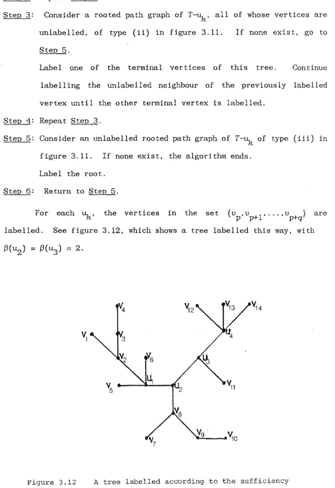
Algorithm 3.1 Any remaining unlabelled vertices of the spanning tree T are labelled u

1,u2, ... ,u n-m-2 as

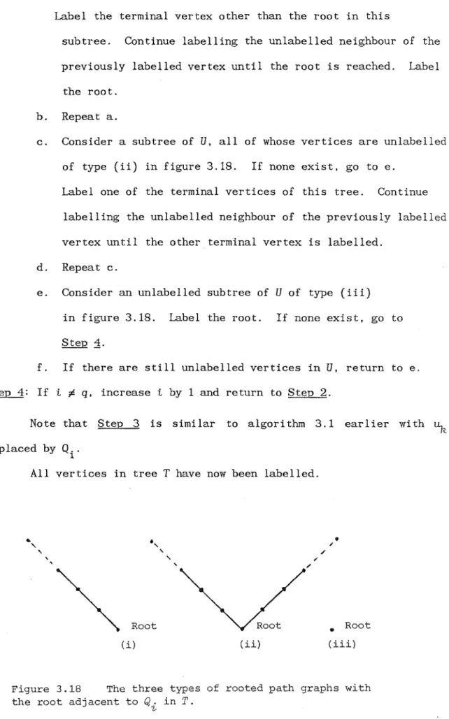
follows:-Step 1: Consider a rooted path graph of T-~, all of whose vertices are unlabelled, of type (i) in figure 3.11. If none exist, go to Step 3.

Label the terminal vertex other than the root in this subtree. Continue labelling the unlabelled neighbour of the previously

Step 2: Repeat Step 1.

Step 3: Consider a rooted path graph of T-~, all of whose vertices are unlabelled, of type ( ii) in figure 3. 11 . If none exist, go to Step 5.

Label one of the terminal vertices of this tree. Continue labelling the unlabelled neighbour of the previously labelled vertex until the other terminal vertex is labelled.

Step 4: Repeat Step 3.

Step 5: Consider an unlabelled rooted path graph of T-~ of type (iii) in figure 3.11. If none exist, the algorithm ends.

Label the root. Return to Step 5.

For each ~· the vertices in the set {v ,vp+l' .. . ,v _{p p+q} } are labelled. See figure 3.12, which shows a tree labelled this way, with

The tree

T

is now redrawn with its vertices in two lines across the page; v

1,v2, ... ,vn-m-2 in order in the upper line and u1,u2, ... ,um+2 in order in the lower. If the tree is drawn with the vertices evenly spaced along the lines, and the edges represented by straight lines, no lines cross improperly since the v. vertices belonging to any ~ occur

l. . R.

consecutively and,the groups occur in the.same order as the~·

Add edges to tree

T

in the following manner:-(i) join u

1 to v1, if not already adjacent;

(ii) join um+₂ to vn-m-₂• if not already adjacent; and (iii) join each vj to vj+

1' if not already adjacent, for each j from 1 to n-m-3