MASTER THESIS
FLOOR VIBRATION
ISOLATION OF A CORIOLIS
MASS-FLOW METER USING
FILTERING TECHNIQUES
K.L.J. Stroeken
EEMCS/SC
MECHANICAL AUTOMATION AND MECHATRONICS
EXAMINATION COMMITTEE
Dr.ir. R.G.K.M. Aarts Dr.ir. W.B.J. Hakvoort Dr.ir. F. van der Heijden
DOCUMENT NUMBER
WA - 1505
SAMENVATTING
In dit onderzoek is de onderdrukking van vloertrillingen en andere verstoringen met behulp van filtertechnieken en additionele sensoren onderzocht. Een door Bronkhorst gemaakte Coriolis Massa-Flow Meter (CMFM) voor kleine massa-flow is gebruikt om inzicht te krijgen in de werking van dergelijke filters. Het verbeteren van deze CMFM bestaat uit twee stappen. Allereerst wordt een voorspelling gedaan van de invloed van de verstoringen op de meetfrequentie. Hierna worden de overige verstoringen zo goed als mogelijk weg gefilterd uit het meetsignaal.
In het eerste deel, de voorspelling, zal eerst een overdrachtsfunctie van vloertrillingen naar massa-flow worden bepaald. Met deze overdracht wordt er een model gemaakt op basis van toestandsvergelijkingen. De gemeten vloertrillingen worden dan met behulp van deze vergelijkingen omgezet in een geschatte massa-flow fout. Na het aftrekken van de geschatte fout van het massa-flow meetsignaal is er bij voldoende vloertrilling een verbetering te zien in de gemeten flowwaarde van 20dB.
ABSTRACT
In this research, narrow-band floor vibration isolation using filtering techniques was evaluated. A Bronkhorst Coriolis Mass Flow Meter, CMFM, for low flows is used as a platform for testing the rejection of the effect of external disturbances on the measurement signal. The robustification of this CMFM consists of both predicting the disturbance at the sensing frequency and removing as much of the other disturbances as possible.
The first part, the prediction, starts with estimating the transfer from floor vibrations to mass- flow measurements. Once this transfer is obtained, it is modeled using a state space model. The measured floor vibrations are fed to this model and then subtracted from the measured mass-flow. This technique attenuates the influence of floor vibrations on the measured mass-flow by 20dB.
PREFACE
The last project for obtaining a Master of Science degree is an individual project of 40 European
Credits. Before I’m going to tell you about what I did in this research, I want to give you a little
insight into the way I got here.
I remember being a little scared and excited coming to Enschede as a “feut” to start studying Electrical Engineering. Since I’m from the south of the Netherlands, a hamlet called Nieuw Bergen, I had to look for a room. I was lucky to find one in the best student residence on campus: “CLUB 9-2”. After an awesome ten days introduction period of partying and getting to know my
fellow students, the first lectures hit me hard; this wasn’t high school anymore! Eventually, after
some warming up I had no real trouble finishing my Bachelor Degree.
Then what?! Then you get to choose again. This time I had to make a decision on which Master program and courses I was going to follow. I already had some work experience in Mechanical Engineering and decided that was the way to go. In consultation with Ronald Aarts, he and I decided that if I followed the Master Systems and Control with some Mechanical Engineering courses, I could finish this Master at the Mechanical Automation chair. The courses were a lot more interesting than the Bachelor courses and especially the projects were great fun.
After finishing up the courses, it was time to show the people what I had learned over the years. For me, this started by going abroad to participate in an engineering internship in Colombia. A project focused on the modeling and control of two parallel manipulators was a nice challenge, which I finished with good result. After spending a few more weeks on vacation in this amazing country, it was time to get back and start graduating.
I found this assignment, that combines Electrical and Mechanical Engineering, challenging. Picking up on a research that started in 2003 is not easy. Luckily Bert, my daily supervisor, had some really neat preliminary research and after some trial and error, I was able to contribute to the project.
Finally after 7 months of hard work and getting used to the 9 to 5 working hours, this report is
laying on my desk. It’s too bad that this also means the end to an era of studying and fun (not
necessarily in that order), but I feel ready and excited to look for a new challenge.
For you, dear reader, the next challenge will be reading all of the things I’ve put down here,
TABLE OF CONTENTS
Samenvatting ... I Abstract ... II Preface ... III Table of Contents ... IV
1 Introduction ... 1
2 Theory ... 3
2.1 Coriolis Mass Flow Meters ... 3
2.2 Disturbances ... 8
2.3 Transfer Function ... 10
2.4 Prediction Filters ... 11
2.5 Band-Pass Filters ... 14
3 Implementation and Results ... 17
3.1 Experimental Setup... 18
3.2 Gain Estimation ... 20
3.3 Prediction Filter ... 21
3.4 Notch Filter ... 24
4 Conclusion ... 28
5 Discussion ... 29
References ... 30
Appendix A: Phase Locked Loop ... 31
1
INTRODUCTION
For continuous production and batch processes, for instance in the pharmaceutical industry, it is sometimes necessary to measure small mass quantities of liquids and gasses. To correctly measure such small mass-flows, a sensor is being developed by Bronkhorst High-Tech based on the Coriolis principle. This type of sensor is able to directly measure mass quantity passing through a tube. Currently there are Coriolis devices commercially available that measure flows as small as 1g/h (1).
However, there is a problem with the further scaling down of these devices. External vibrations from pumps or other equipment generate measurement errors. The cause for this is the fact that the measured Coriolis force, induced by a mass-flow, cannot be distinguished from forces caused by vibrations. Measurement errors increase as the Coriolis force decreases more from scaling down than vibration forces.
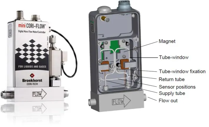
[image:6.595.86.441.377.593.2]Currently, there is research being done to make Coriolis Mass Flow Meters, or CMFMs, less vulnerable to external vibrations. There are projects that focus on passive and active vibration isolation removing disturbances from the tube (2). These solutions however, are costly and can add asymmetry to the device resulting in an incorrect flow measurement.
FIGURE 1 - BRONKHORST CORIOLIS MASS FLOW METER (LEFT) AND DETAILED SKETCH (RIGHT)
In this research, the CMFM in figure 1 is robustified by measuring the external vibrations, predicting their effect on the flow measurement and correct for it. Therefore, no extra stages are added to the measurement device.
2
THEORY
In this chapter some theoretical background of the sensor workings is explained before taking a closer look at the disturbances acting on the sensor. These paragraphs are mainly based on prior research (1), (3) and (4). In the third paragraph the first added work is seen in the form of deriving the transfer function from the disturbances to the measurement error after which this information is used for the prediction filter in paragraph 2.4. The last part of this chapter explains the contribution and workings of a band-pass filter.
2.1
CORIOLIS MASS FLOW METERS
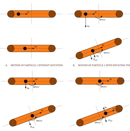
Before going more into detail on the research, the workings of a Coriolis Mass Flow Meter are explained. The measurement principle of CMFMs is based on the acceleration and deceleration of a moving mass in a rotating frame. For the sake of explaining this principle, the motion of three particles through a rotating tube is examined. A top view of the tube is depicted in figure 2.
A. MOTION OF PARTICLE 1 WITHOUT ROTATION B. MOTION OF PARTICLE 1 WITH ROTATING TUBE
[image:8.595.70.522.297.754.2]C. MOTION OF PARTICLE 2 WITH ROTATING TUBE D. MOTION OF PARTICLE 3 WITH ROTATING TUBE
In figure 2a, a mass-flow from left to right is depicted by a particle moving through a tube with a
constant flow velocity . The upper tube of figure 2a displays the position of the particle at t=0.
At the next time instance, displayed in the lower half of figure 2a, the particle moved towards the right representing mass-flow. Next, the tube is rotated around its center with a constant angular
velocity . Again the upper pictures show the state at t=0 and the lower pictures show t=1;
the next time instance.
For particle 1 this is seen in figure 2b. The upper figure shows that due to the angular velocity of
the tube, , particle 1 has a velocity at t=0. At the next time instance, t=1, the tube rotated
and the particle moved towards the axis of rotation due to its flow velocity . As the angular
velocity remained constant and the particle moved towards the axis of rotation the velocity decreased. By Newton’s law this deceleration caused a force on the tube called the Coriolis force and depicted by .
The same can be seen for particle 2 in figure 2c. This particle also moves towards the center of
the tube. Just like particle 1 the particle velocity due to the angular velocity decreases during
this movement. This causes a similar Coriolis force on the tube, as the deceleration is equal. In figure 2d, a third particle is now moving away from the axis of rotation. As it moves away, the
particle velocity now increases due to the constant angular velocity and an increased
distance from the center of rotation. This also causes a reaction force on the tube in the
opposite direction of the acceleration. It should be noted that the direction of the accelerating particle causes a force in the same direction as the force of the decelerating particles. Summing
over all particles, the rotating tube experiences a Coriolis force proportional to the
mass-flow .
The magnitude of the Coriolis force is calculated using the acceleration and mass of each moving
particle and summing over all particles in the tube. Each particle velocity is given by
(2.1)
where is the position of the particle relative to the center of rotation. The particle acceleration
can be written as the derivative of (2.1)
(2.2)
Next, the Coriolis force acting on the tube is calculated using the particle mass . Note that this
force has an opposite direction than the force acting on the accelerating particle.
(2.3)
Now, instead of looking at one particle, there is a continuous flow consisting of infinite small
particles. The tube has a length, L, and sectional area, A. Here, is used as the integration
variable over the tube length and represents the infinite small length of a cross-section of the
where is the mass-density of the flow. Integrating over the length of the tube gives
∫
(2.5)
Now, instead of a continuously rotating tube, it is much easier to construct an oscillating tube. The principle of the Coriolis effect still holds. This effect generates a force on the tube proportional to the length of the rotating tube, the mass-flow and the angular velocity. From
(2.5) and recognizing as the mass-flow, ̇, the Coriolis force on the tube can be written as
̇ (2.6)
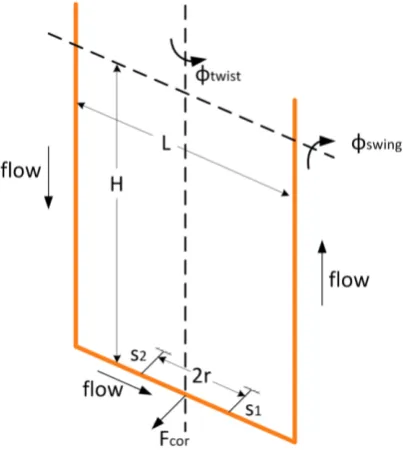
[image:10.595.71.273.349.575.2]This Coriolis force arises at a tube section normal to the rotation axis. Simultaneously, its direction is perpendicular to the tube window as can be seen in figure 3. Here the tube section examined in figure 2 is the lower part of the tube window.
FIGURE 3 - THE TUBE WINDOW
The generated Coriolis force causes tube motion around the swing axis of the tube window with the same frequency as the actuated twist motion. The swing motion caused by the Coriolis force is 90 degrees out of phase with the actuation. This is because a force proportional to the velocity of the actuation motion actuates it. Two sensors are placed on opposite sides of the actuation axis measuring both actuation (twist) and swing (Coriolis) motion. For small motions the sensor signals are almost equal to
(2.7)
(2.8)
where is the actuation frequency. According to (2.6) the actuated motion will cause a
Coriolis swing motion proportional to the mass flow
̇ (2.9)
Using (2.7), (2.8), (2.9) and some trigonometry the time-varying sensor signals can be written as
(2.10)
where if no mass is flowing through the tube and thus no Coriolis motion is
generated. This is due to the sensors being at opposite sides of the twist axis.
The contribution of (2.9) to (2.10) gives an extra, opposite phase shift between and in
and . This phase shift is a direct measure of the amount of mass flowing through the tube.
Multiplied with a sensor sensitivity, , there is a linear approximation between the mass-flow
and the phase difference which holds for small phase angles
̇ (2.11)
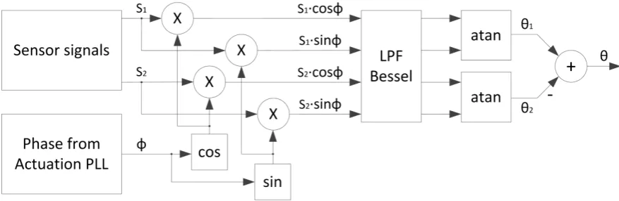
[image:11.595.70.509.467.610.2]where the sensor sensitivity is based on material properties and tube window dimensions. A Dual Quadrature Demodulation scheme (DQDM) (3) is used to measure the phase difference between the two sensor signals.
FIGURE 4 - DUAL QUADRATURE DEMODULATION SCHEME
Mixing generates two signals; one with the original frequency subtracted from the mixing frequency and one where the signal frequency is added to the mixing frequency
( ) ( ) (2.12)
In this case mixing is done with the signal frequency, resulting in a DC component of the signal and the second harmonic of the signal frequency.
For the first sensor signal the result after mixing is written as
( ) (2.13)
( ) (2.14)
Applying a low pass filter (LPF) to the mixed signals removes the second harmonic. A Bessel filter is used as it has a constant delay for all pass-band frequencies. This means that no matter the change rate of the flow there is a constant delay in the filter. Therefore, the total flow is most correctly calculated.
Low-pass filtering (2.13) and (2.14) gives
( )
⇒ (2.15)
( ) ⇒ (2.16)
the arctangent of the filtered signals gives the phase of the sensor signal
(
) (2.17)
where the calculated phase does not depend on the signal amplitude c.
The same path is followed for the second sensor signal giving the phase . From (2.11) and the
2.2
DISTURBANCES
In this paragraph, the effect of external vibrations on the measurement error of Coriolis mass-flow meters is explained. To this end the disturbance directions are identified and their effect on the measurement is evaluated. Also, the sensor placement for measuring the correct disturbances is discussed.
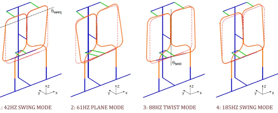
In a prior research done by Van de Ridder (4), the major disturbance directions of CMFMs were identified. In that research a model of the sensor window was constructed using the multi-body modeling tool SPACAR (5). In figure 5, the first four eigenmodes of this model are depicted and their natural frequencies are given. It should be noted that the Coriolis force causes a swing motion at the frequency of the actuation (twist) mode and although it causes similar motion it does not excitate the first swing mode in its eigenfrequency. The frequencies in figure 5 can change by a maximum of plus or minus five percent due to flow density and temperature differences. The filtering algorithms should be able to cope with these varying frequencies.
[image:13.595.74.520.299.481.2]1: 42HZ SWING MODE 2: 61HZ PLANE MODE 3: 88HZ TWIST MODE 4: 185HZ SWING MODE
FIGURE 5 - THE FIRST FOUR MODESHAPES AND CORRESPONDING EIGENFREQUENCIES OF THE WINDOW
A multi-sine (1-550Hz) in all six degrees of freedom has been presented to the casing while the flow, was measured. By using the floor accelerations and flow measurements, a transfer was estimated from each disturbance to the measurement value. It showed that a disturbance in the y-direction had 50dB more contribution to the measurement error than any other disturbance. This is understood when noticing that the displacement caused by the Coriolis force is the same as the first swing mode. It is easy to see that the first swing mode is excited by a rotation around the x-axis or a y-displacement. Experiments show that y-displacements have a much larger contribution than x-rotations.
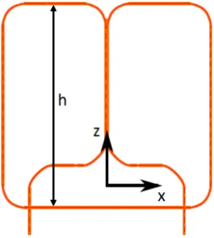
As stated, the sensor should be able to measure y-disturbances. The position where these disturbances play the biggest role is in the tube window’s center of moving mass for the first
swing mode. This location is at a z-position 5% of the height of the tube window depicted in
[image:14.595.75.232.175.349.2]figure 6. At this position, disturbance rotations about the x-axis that contribute to the measurement error are also measured as y-displacements, making it the ideal position. By placing the sensor in this point maximum attenuation can be achieved with only one sensor.
FIGURE 6 - SENSOR PLACEMENT
The x-position of the sensor has to be on the twist axis i.e. the center of the tube window. This ensures that no actuation motion is measured.
The sensor-type is an acceleration sensor as this is the most convenient device for measuring disturbances.
2.3
TRANSFER FUNCTION
In this paragraph, the transfer from disturbances perpendicular to the tube window, , to
Coriolis displacement is derived. In figure 7, a simplified disturbance model is shown. Despite
[image:15.595.230.526.292.631.2]its simplicity it is a good model of the system, as only one disturbance direction and mode are dominant in the effect of external vibrations on the flow measurement.
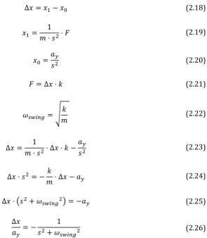
FIGURE 7 - SIMPLIFIED MODEL FOR DERIVING THE TRANSFER FROM VIBRATIONS TO CORIOLIS DISPLACEMENT From this model the transfer function is derived
(2.18)
(2.19)
(2.20)
(2.21)
√ (2.22)
(2.23)
(2.24)
( ) (2.25)
(2.26)
Conversion of and to volts in the setup, gives rise to a scaling factor . The total transfer
from floor accelerations to Coriolis displacement is then given by
(2.27)
2.4
PREDICTION FILTERS
With the transfer from paragraph 2.3, a prediction filter is built that estimates the influence of the disturbances and directly subtracts them from the measurements. Recall from section 2.2, that disturbances are only important at the actuation frequency. This is the frequency at which the Coriolis displacement is measured and therefore no information should be removed by band-pass filtering. A prediction filter can in this case present a solution as it does not blindly
filter the signal, but makes a prediction of the disturbance’s influence. This prediction can then
[image:16.595.71.417.213.303.2]be subtracted from the measured sensor signal to enhance the system output.
FIGURE 8 - GENERAL PREDICTION FILTER
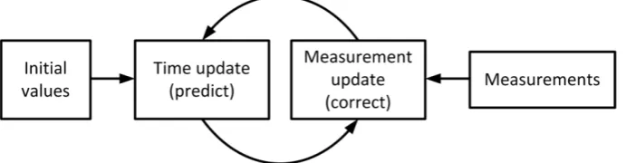
Prediction filtering is a two-step recursive process as seen in figure 8. First, a prediction is executed based on model information, i.e. the transfer function, the current description of the system; the system’s state vector and the input accelerations. During this prediction a state uncertainty matrix is updated. This uncertainty matrix describes the correctness of the state
vector. In this case, the new state vector’s uncertainty is updated with the model uncertainty.
This increases the uncertainty of the state vector, as the model is almost never 100% correct. The second step of prediction filtering is a correction. This update happens when a new measurement is available. During correction the measurement and the prediction are compared and the difference between them is used to calculate the innovation. The innovation describes the amount by which the new system state is corrected. This innovation is based on the measured difference between the state vector and the measurement with both the measurement and the state uncertainty taken into account. If the measurement uncertainty is much greater than the current system state uncertainty, only a small amount of the measured difference is added to the system state vector. If the measurement is more certain than the state, a large amount of this difference is added. This process continuously estimates the best possible system state vector and suppresses the influence of noise. After correction a new state uncertainty is calculated. The state uncertainty after a measurement update always decreases as the measurement adds information. After correction a new prediction is done.
Kalman filters require the system transfer function to be written in state space form
(2.28)
with
The transfer function (2.27) is used to obtain the system transition matrix F and input matrix L. The state space transfer function is discretized and the input and transition matrix are calculated. The state space transfer is found to be
[ ̂ ̂ ] [
] [
] [ ] (2.29)
where
̇
The Kalman filter uses equation (2.29) for predicting the next state. A so-called covariance matrix is used to keep track of the uncertainty. The state covariance matrix for the next state
̂ is calculated using the process covariance matrix . resembles the state
uncertainty whereas gives the uncertainty of the model and input signal. The next state
covariance matrix is calculated according to
̂ (2.30)
When a new measurement is available, the current state information is updated with this
information. Using the measurement noise covariance matrix , the innovation matrix is
calculated
̂ (2.31)
where H is the measurement matrix. In this model the position is measured and therefore the measurement matrix is given by
[ ] (2.32)
Using the innovation matrix the Kalman gain matrix is determined
̂ (2.33)
which allows updating the system state vector and covariance matrix using the
measurement of the CMFM’s tube position sensor
̂ (2.34)
The covariance matrices should be initially set to large uncertainties as the start-up state of the system is unknown. This results in large innovations at start-up where the filter relies a lot on its measurements. After some time, the system state becomes more certain and the innovations will decrease. The filter relies more on the transition matrix to obtain its next state. Finally, the Kalman gain matrix will become a steady matrix. This is because of the constant measurement and input covariance gives a constant certainty ratio of measurement and predicted state. Although being constant, the innovation, Kalman gain and covariance matrices are continuously updated. This consumes a lot of processing power just to have faster convergence at start-up. Since the Coriolis Mass Flow Meters are generally used during long-term operation, this recalculation is unnecessary. Therefore a steady state Kalman gain matrix is calculated using the
process, measurement and input covariance matrices and MATLAB’s dlqe command. This
reduces the number of equations for one correct and predict cycle, from six to two: (2.29) and (2.34).
2.5
BAND-PASS FILTERS
Filtering the signal before and during processing can massively improve the signal to noise ratio, SNR, of the final measurement. As explained in paragraph 2.1, the dual quadrature demodulation scheme has a low-pass filter after the mixer to remove noise from the measurement. The
bandwidth of this filter is in direct correlation with the sensor’s response time, e.g. if a 10Hz
wide low pass filter is used, the fastest response time is 0.1s. If this low pass filter is projected at the actuation frequency using (2.12) a 10Hz low-pass filter effectively becomes a 20Hz band-pass filter.
In theory, a wide filter is required to achieve a decent response time after phase calculation. However, the bandwidth of the same response in the time signal is much smaller. This can be seen when looking at the frequency change due to a changing mass-flow. From (2.11) it follows that a mass-flow causes a phase difference. When the mass-flow, and thus the phase changes, a temporary frequency shift is measured in the time signal. For one of the two sensor signals the phase change, and thus the frequency shift, is positive, while for the other it is negative. The shift is equally divided between the two sensor signals. To measure the temporary frequency shifts a bandwidth around the signal frequency is needed. The required bandwidth in the time domain is
calculated from the maximum flow change, , the desired response time, , and the
sensor sensitivity, ,
(2.36)
With a measurement sensitivity (2) of (
), a response time of 0.1 and a maximum flow
change from -100 to 100 the necessary bandwidth can be calculated
(2.37)
Compared to the low-pass filter in the DQDM, the bandwidth needed in the time domain for obtaining the same response is roughly 80 times smaller. If such a filter can be constructed the disturbance rejection is theoretically improved with that same factor, i.e., 38dB.
In practice, band-pass filters for discrete time applications are categorized as either finite impulse response filters, FIR filters, or infinite impulse response filters, IIR filters. FIR filters use only a finite amount of input samples, but are in general more complex than IIR filters. The latter calculate the output value also based on previous output values. This requires less filter coefficients, but results in a filter with infinite memory.
A notch filter is a simple IIR filter and is used to examine the contribution of band pass filters. The notch filter cancels a specific notch frequency and is almost constant at all other frequencies. The transfer function of a second order notch filter (8) is given by
(2.38)
where the parameter is based on the normalized notch frequency, , as
(2.39)
and the normalized bandwidth of the filter is determined by and given by
(
) (2.40)
with . The higher gets, the more selective this filter becomes.
Based on equation (2.38), the notch filter equations can be written as two recursive update equations (9) that can be calculated when a new measurement enters the system. The
intermediate variable is used as the memory variable working on both in- and output
values. The update equations are given by
(2.41)
(2.42)
and the estimated signal is
̂ (2.43)
which represents just the actuation frequency content of the measurement signal
effectively making it a band-pass filter.
The notch frequency of the filter has to be within the range [ ] of the Nyquist
By creating multiple resampled datasets, an easy reconstruction of the signal is possible after applying the notch filter. This can best be seen if the resampling is executed during notch filtering. The update equations (2.41) and (2.42) then become
(2.44)
(2.45)
representing the resampled signal with the actuation frequency content removed. Equation (2.43) can again be used to obtain the signal at the actuation frequency.
3
IMPLEMENTATION AND RESULTS
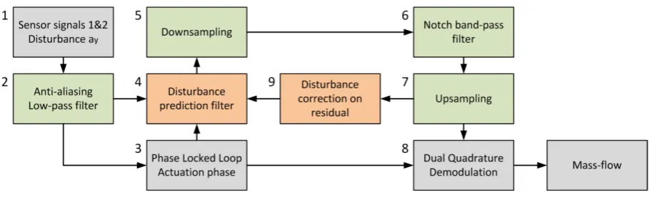
[image:22.595.70.525.260.402.2]In this chapter the theory in the previous chapter is combined into one solution. The filtering algorithms are implemented using MATLAB on a Windows personal computer with a 2,8GHz Intel i7 processor and 4GB internal memory. Datasets with measured disturbances are used to check the workings of the proposed algorithms. During these experiments there is no flow and thus the result of the measurement should be 0. Also, step responses are simulated to check the response time of the proposed algorithms. The gains for the prediction filter are estimated in paragraph 3.2. The flow is calculated using the Dual Quadrature Demodulation scheme explained in paragraph 2.1. This is done for a signal without extra filters and a signal with added prediction and band-pass filtering. The influence of both added filtering techniques is evaluated. The complete signal flow chart of processing the measurements is shown in figure 9.
FIGURE 9 - SIGNAL PROCESSING OVERVIEW
The total signal processing algorithm now has nine steps. First, the sensor signals and the disturbance accelerations are measured using opto-sensors and an accelerometer respectively. Next, the measured signals are low-pass filtered. This ensures there is no aliasing when resampling the signal. Thirdly, the actuation frequency and phase are determined using a Phase Locked Loop (10). The workings of such a PLL are expounded in Appendix A. The fourth step is making a prediction of the disturbance based on the measured accelerations and the estimated transfer. After that, the signal is sampled down to enable correct operation of the notch filter. Here, 32 datasets are created such that the signal can be easily reconstructed without information loss. The sixth step is applying the notch filter on the time signal in an attempt to remove disturbances that are not at the actuation/Coriolis frequency. After that, the 32 signals are stitched back together. Step eight is calculating the flow using the Dual Quadrature Demodulation technique, itself consisting of mixing, filtering and phase calculation. The ninth and last step is correcting the disturbance prediction based on the residual. This is the signal with only disturbances and no actuation content.
3.1
EXPERIMENTAL SETUP
[image:23.595.70.475.177.332.2]For testing purposes, the CMFM is placed on a shaker platform with six degrees of freedom (DOF) (11). This Stewart type suspended platform is actuated by voice coil motors. Co-located acceleration sensors (Endevco7703A-1000) measure the applied disturbances. These disturbances are transformed from the acceleration sensor locations to the Cartesian coordinates depicted in figure 10 using a rigid body model. The setup is shown in figure 10.
FIGURE 10 - EXPERIMENTAL SETUP: THE CMFM ON THE SHAKER
The disturbance forces are measured using the accelerometers. The response of the CMFM to the disturbances is measured using the opto-sensors also used for measuring mass-flow. Both the accelerometers and the opto-sensors use a National Instruments NI4472 data capturing device able to measure 8 channels with a 24-bit resolution at a sample rate of 24kHz. 60 seconds of data is captured during each experiment. Experiments are executed with and without the CMFM flow-measurement enabled and for varying disturbance levels.
FIGURE 11 - APPLIED DISTURBANCE SPECTRUM
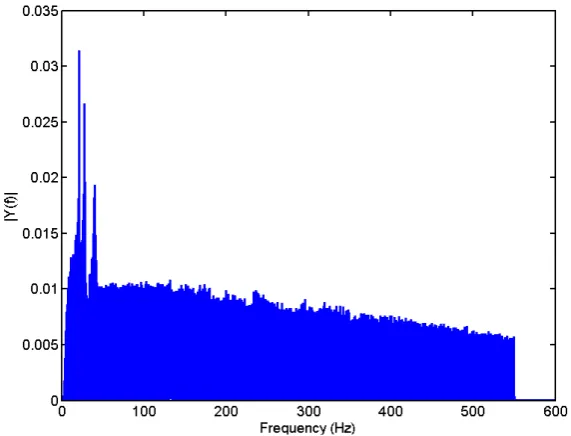
[image:23.595.70.356.458.676.2]In order to gain a little more insight, the signal frequency spectrum of the opto-sensors is depicted in figure 12. Here, the CMFM is turned on, i.e. the twist mode is actuated, enabling flow measurements.
FIGURE 12 - FREQUENCY SPECTRUM OF THE OPTO-SENSOR SIGNALS
In figure 12 it can be seen that there is a huge peak at the actuation frequency of 88Hz. Also, some signal content is seen at 42Hz. This is the first swing mode, which is excited by the
disturbances. Some smaller disturbances are seen at 23Hz, the shaker’s eigenfrequency, 61Hz,
the second Eigenmode of the tube, and 185Hz, the second swing mode. These disturbances have almost no influence on the measured flow and will therefore be ignored.
Recall from paragraph 2.2 that only the measured disturbances in y-direction are used. These have 50dB more contribution to the flow error than any other disturbance. The y-direction is seen from the CMFM coordinate frame. In figure 10 the coordinate frame is depicted.
In the next paragraph, the CMFM will be turned off, i.e. the twist mode is not actuated, in order to
come up with a disturbance model from y-disturbances, , to swing motion. In paragraph 3.3,
3.2
GAIN ESTIMATION
The y-disturbances and the swing motion are measured for 60 seconds. The transfer function,
from applied disturbances to Coriolis displacement, is estimated using MATLAB’s system
identification toolbox, Ident. For this purpose actuation of the CMFM is turned off, such that only the motion caused by the floor vibrations is measured.
The measured data are translated to Cartesian coordinates and imported in Ident. After detrending the data, a second order state space model is estimated. There are two opto-sensors in the CMFM, so this is done twice ultimately giving two transfer functions. These estimated transfer functions are then compared to the derived transfer (2.26). This is shown in figure 13. Before the estimated transfers are evaluated, recall from paragraph 2.1 that only disturbances around the actuation frequency are of interest. The actuation frequency lies at 88Hz or 553rad. At this frequency, the response in (2.27) simplifies to
(3.1)
[image:25.595.71.370.382.622.2]meaning that the transfer is mostly affected by a changing actuation frequency and not by a change in the swing frequency, i.e. a change in the third instead of the first eigenmode (see paragraph 2.2).
FIGURE 13 - ESTIMATED TRANSFERS FROM FLOOR ACCELERATIONS TO CORIOLIS DISPLACEMENT
It can be seen that there are two deviations between the estimated transfers and the model. Firstly, the system is modeled without any damping, but the real system has a little damping. This does not influence the transfer at the actuation frequency and is therefore not important. Secondly, the gain is not correct in the estimated model. The gain parameter of the derived transfer (2.26) was set to -1. The correct gain is calculated by dividing the derived gain by the
3.3
PREDICTION FILTER
As stated in paragraph 2.4, disturbances at the actuation, and thus Coriolis frequency, are rejected by predicting the influence of external vibrations at this frequency. In this paragraph, the workings of this prediction filter are tested without the influence of a band-pass filter. A summary of the algorithm is depicted in figure 14. Due to practical restrictions, a notch filter is implemented, but only for calculating the residual used for the measurement update. This filter does not enhance the processed signal.
The filter is implemented with the gains from the previous paragraph and a process covariance based on an estimated model uncertainty of 1 percent. The measurement correlation value is 0.001, which is equal to the actual noise level. From these uncertainties, the measurement matrix (2.32) and the state transition matrix (2.29), the steady Kalman gain matrix is calculated and found to be
[ ] (3.2)
Despite the high sampling rate, the found values for are rather low. This indicates that the
[image:26.595.69.530.369.502.2]filter relies on the model and assumes that information to be correct. This also means that measurement corrections are small.
FIGURE 14 - FLOW CALCULATION WITH PREDICTION FILTERING
The disturbances measured by the acceleration sensor are fed to the prediction filter. The sensor gains found in paragraph 3.2 of -644 and -539 for sensor 1 and 2 respectively are used in the input matrix of (2.29). The flow is calculated using the DQDM scheme from section 2.1.
The result of the Kalman filtering is seen in figure 15. This filter gives 17.3dB disturbance attenuation on the measured flow. This is calculated by comparing the standard deviations of both the filtered and the unfiltered flow. It took 27 seconds to execute this filtering on 60 seconds of data.
Decreasing the uncertainty of the model increases the attenuation. By changing the model uncertainty to 0.1 percent a steady Kalman gain matrix becomes
[ ] (3.3)
Although notch filtering removes almost the entire actuation signal, some is still left in the measurements. When information at the actuation frequency is fed to the Kalman filter it is seen
[image:27.595.72.354.123.351.2]as an external disturbance and therefore the filter removes a signal that originally wasn’t there.
FIGURE 15 - FLOW BEFORE AND AFTER REMOVING THE KALMAN PREDICTED DISTURBANCE
Furthermore, disturbances at other frequencies than the actuation frequency are not important for the Kalman filter since they are later removed by either the notch filter or the low-pass filter in the DQDM. With this in mind, the correction is disabled, i.e. the Kalman gain is set to zero, such that no measurement updates occur. To prevent the estimated signal from growing unbounded, a little damping is added to the state transition matrix. The damping factor is based on the high Q-factor of the system. However, due to sensor noise the damping value cannot be too small as this noise continuously adds energy to the filter. The damping can be seen as the factor smaller than 1 by which the velocity is multiplied to obtain the new velocity. The new state transition matrix now becomes
[
] (3.4)
Disabling the update improves the disturbance attenuation to 19.2dB and reduces processing time to 22 seconds.
Next, the gains found in paragraph 3.2 are altered to check whether they are optimal. Some
tuning finally gives a 20.7dB attenuation for gains of and for sensor 1 and 2
respectively.
To gain some more insight in the effect of a mismatched gain, some experiments are done in
which this gain is varied. The result on the filter’s attenuation is plotted versus a gain error
From figure 16 it can be seen that a gain match within 3% of the actual gain is sufficient for estimating the disturbance influence. When the gain is known accurately, there are other causes why the attenuation no longer increases. These causes can be found in the noise levels of the sensors. For this test, the calculation of the y-acceleration is based on multiple sensors causing errors to add up.
FIGURE 16 - GAIN ERROR VERSUS FILTER ATTENUATION
When the disturbance level decreases, the filter has less attenuation. If no intentional external disturbances are presented to the CMFM, the prediction filter still improves the measurement value by 0.2dB. The measured disturbance level with no intentional external vibrations has an
order of magnitude of . It is also noted that the prediction filter adds no delay
whatsoever to the response.
3.4
NOTCH FILTER
[image:29.595.71.526.144.280.2]A notch filter is implemented for filtering disturbances around the actuation frequency. The prediction filter is disabled. The processing algorithm with only a notch filter is summarized in figure 17.
FIGURE 17 - FLOW CALCULATION WITH NOTCH FILTER
The implemented filter has a bandwidth of 0.34Hz. This is the theoretically required bandwidth from (2.37) with 0.1Hz extra uncertainty from the actuation frequency estimation. The 0.34Hz
bandwidth corresponds to . The notch-filtered result is compared to a flow
[image:29.595.72.353.373.595.2]calculation without notch filter called the measurement. The result can be seen in figure 18.
FIGURE 18 - THE NOTCH FILTERED FLOW COMPARED TO THE MEASUREMENTS
As the notch filter is a resonance filter with memory, it is interesting to check the response time. The filter’s response to a step change in the flow is simulated. The result of this simulation for a 0.34Hz bandwidth can be seen in figure 19.
FIGURE 19 - RESPONSE OF THE NOTCH FILTER TO A STEP RESPONSE IN THE FLOW AT T=45S
The step in figure 19 shows that the response time of the filter is in the order of 20 seconds. This is the time at which the filter reaches its final value plus or minus 1 percent.
To further evaluate the notch filter, its bandwidth is compared to the response time and depicted in figure 20.
FIGURE 20 - NOTCH FILTER BANDWIDTH VERSUS RESPONSE TIME
[image:30.595.71.351.449.668.2]The relation between filter bandwidth and attenuation is also interesting. This is depicted in figure 21.
FIGURE 21 - NOTCH FILTER BANDWIDTH VERSUS ATTENUATION
From this figure, it can be seen that the aforementioned 10Hz filter bandwidth corresponds to 6dB attenuation.
A variable can be added to the notch filter which checks whether the filter still correctly filters the signal (9). This variable can simply check if the output of the filter has more signal content than the removed disturbances. If it does, the bandwidth can be reduced towards its theoretical minimum of 0.34Hz. If this variable indicates that the filtered signal is not correct, the bandwidth is immediately set to 10Hz in order to obtain the required response. This ensures that the filtered signal contains the flow information while achieving maximum attenuation. In general, it can be stated that higher order filters introduce a larger delay. Also, the smaller the pass-band, the larger the delay becomes. There is always a trade-off between delay and noise attenuation. The adaptive notch filter, that can vary both the notch frequency and the filtered bandwidth, is a good solution to this problem. This enables maximum noise attenuation for a stable flow and a fast response for varying flow signals.
The filter’s robustness against varying actuation frequencies is checked and it is found to track changes up to 4Hz per second.
When adding a prediction filter to the notch filter, the total result of the algorithms is found. Here, a notch filter width of 10Hz is used. The flow result after applying prediction and notch filtering is seen in figure 22.
FIGURE 22 - PREDICTION AND NOTCH FILTERED FLOW COMPARED TO THE UNFILTERED FLOW
4
CONCLUSION
From this research on the attenuation of external vibrations using filtering techniques, two conclusions are drawn. The results are summarized in table 1.
[image:33.595.67.529.298.419.2]Firstly, with the prediction of the influence of external vibrations by a Kalman filter, an attenuation of 20.7dB is achieved. For this filter to operate properly, the gain at the actuation frequency has to be known. This was determined by estimating the transfer function from floor vibrations to the measurement error. The measurement update of the filter should be disabled if the measurements for correction have signal content at the actuation frequency. This causes the filter to base its estimation on non-existing disturbances, which worsens the filter output and can eventually even worsen the measured mass-flow.
TABLE 1 - OVERVIEW OF THE DISTURBANCE ATTENUATION PER FILTER
Response
time -
Kalman Kalman Kalman Kalman
- 0.1s 0dB -20.7dB -15dB -8.1dB -0.2dB
Notch 10Hz 1s -6dB -22.1dB
Notch 0.34Hz 20s -24.5dB -40.3dB
Secondly, time domain filtering can massively improve the signal to noise ratio of the measured signal. The required bandwidth for filtering the sensor signals is theoretically 80 times smaller than for filtering the calculated phase. Therefore, in theory 38dB attenuation can be achieved. A notch filter of 0.34Hz showed 24.5dB improvement in practice, but as it is a resonance filter the response time was over 20 seconds. This can be solved by letting the filter converge towards a small bandwidth and check if the filtered signal has no actuation signal content. This is done by
increasing the -parameter. If the signal is lost, the notch bandwidth is set to 10Hz. This
attenuates the noise by 6dB while obtaining a desired response time of 1s.
5
DISCUSSION
This research showed that it is possible to obtain a reasonable attenuation of external disturbance using a prediction filter. The notch filter however, caused an undesired large response time. Therefore, it is interesting to look further into filtering the sensor signals in the time domain. For instance, adaptive FIR filtering with a small pass-band around the actuation frequency can be an option. Although this costs a lot of computational power, band-pass filtering creates a theoretical improvement of the SNR of 38dB.
Furthermore, it is known that the tube window’s rotation pole (the point on the bottom tube
around which the window twists) shifts from the expected twist axis. With the sensor gains known, the rotation pole of the tube window can be calculated based on the measured signal amplitudes. The PLL is able to estimate these amplitudes and, as the positions of the sensors are known, the rotation pole has a simple linear relation with the measured signal amplitude. Also, if the location of the rotation pole is known, this can be used to improve the disturbance estimate. The disturbance sensor is in the center of the CMFM. If the rotation pole is not exact in the center, this causes some of the actuation signal to be measured by the disturbance sensor. This has no real influence on the flow measurement and therefore it should not be in this estimated disturbance. It can be removed by measuring the actuation amplitude, the position of the rotation pole and the mass of the tube compared to the case. This gives a transfer from actuator motion to disturbance sensor by which the influence of actuator motion can be eliminated.
Another remark has to be made on the attenuation of crosstalk. If two CMFMs are placed close together the actuation signal of the one CMFM acts as an external vibration on the other CMFM and vice versa. As the actuation frequencies of similar devices are almost equal, this disturbance cannot be removed by regular filtering. The prediction filter presents a very good solution in this case as the crosstalk disturbance is measured by the acceleration sensor and can thus be attenuated.
Furthermore, the prediction filter works better if more disturbance is present. That way the noise level of the acceleration sensors play a less crucial role and thus more attenuation can be achieved. It should be noted that for this to be true, the gains have to be determined accurately. However, the filter still attenuates disturbances if no intentional external disturbances are presented to the CMFM.
Instead of adding extra band-pass filters, also an attempt could be made to construct a varying low-pass filter in the DQDM scheme. This filter can also converge for steady flows and react to a flow change by increasing the bandwidth.
The last remark is made on the actuation frequency. A higher actuation frequency allows for easier filtering. Due to the mixing, the low-pass Bessel filter can more easily remove the disturbance frequencies if they are further away from the actuation frequency in an absolute
sense. This doesn’t hold for the notch filter. With an increased actuation frequency the total
REFERENCES
1. Anklin, M. Coriolis mass flowmeters: Overview of the current state of the art and latest
research. Flow Measurement and Instrumentation. 2006, Vol. 17, 6, pp. 317-323.
2. Ridder, L. van de. Active vibration isolation feedback control for Coriolis Mass-Flow Meters.
Control Engineering Practice. 2014, Vol. 33, pp. 76-83.
3. —. Quantification of the influence of external vibrations on the measurement error of a
Coriolis mass-flow meter. Flow Measurement and Instrumentation. August 29, 2014, pp. 39-49.
4. Mehendale, A.Coriolis Mass Flow Meters For Low Flows. Enschede : Print Partners Ipskamp,
Enschede, 2008.
5. Aarts, R. and J. Meijaard, J. Jonker. SPACAR 2013 - Manual. University of Twente. [Online]
March 14, 2011. [Cited: 10 14, 2014.]
http://www.utwente.nl/ctw/wa/software/spacar/2013/manual/.
6. Heijden, F. van der. Classification Parameter Estimation & State Estimation An Engineering
Aproach Using MATLAB. West Sussex PO19 8SQ, England : Wiley, 2004.
7. Yuan, J. Adaptive Laguerre filters for active noise control. Applied Acoustics. 2007, Vol. 68, pp.
86-96.
8. Ciochină, S. Adaptive Notch IIR Filters an implementation on Motorola SC140. Bucharest,
Romania : University of Bucharest, Faculty of Electronics and Telecommunications, 2003.
9. Shen, T. A Novel Time Varying Signal Processing Method for Coriolis Mass Flowmeter. Review
of Scientific Instruments. 065116, 2014, Vol. 85.
10. Wu, B. A Magnitude/Phase-Locked Loop Approach to Parameter Estimation of Periodic
Signals. IEEE Transactions On Automatic Control. 2003, Vol. 48, 4, pp. 612-618.
11. Tjepkema, D. Active hardmount vibration isolation for precision equipment. Enschede :
APPENDIX A: PHASE LOCKED LOOP
In this research, some Phased Locked Loops, PLLs, were used for estimating phases and frequencies. Here, the workings of such a PLL are explained.
[image:36.595.72.447.274.464.2]In general, a PLL is used to estimate or track the parameters of a slowly varying periodic signal. In this case, the actuation signal is tracked by a PLL. This is done for 3 reasons. Firstly, the force actuator for the twist mode requires the phase of the actuator motion in order to actuate correctly. The reason for this is found in the fact that the tube is actuated in resonance such that a large actuation amplitude can be obtained with little actuation energy. Secondly, the signal processing uses the actuator phase for mixing and predicting. Furthermore, the notch filter requires the signal frequency to assure setting the correct notch frequency. All of this information is gathered by a PLL.
FIGURE 23 - PHASE LOCKED LOOP
The PLL extracts the frequency , phase and amplitude (10) from a periodical
signal. The scheme in figure 23 is used to derive the PLL update equations. Note that the system
is discretized which requires an estimated ̂ for causality.
̂ (0.1)
(0.2)
(0.3)
( ) (0.4)
̂ (0.5)
( ) (0.6)
where the design parameters , and determine the trade-off between convergence time
and disturbance rejection for respectively the amplitude, frequency and phase. is the sample
The parameter should be as low as possible, as it is a direct feed through for disturbances. The other parameters are also tuned to be as low as possible, but have to able to track a 4Hz frequency change per second, at the typical resonance frequency of 88Hz, and a step change in the flow. The parameters are found to be
(0.7)
(0.8)
(0.9)
The PLL is capable of tracking the actuation frequency, , within 0.05Hz, even when
[image:37.595.71.358.271.491.2]disturbances are presented to the CMFM. This is depicted in figure 24.
FIGURE 24 - ESTIMATED ACTUATION FREQUENCY WITH EXTERNAL DISTURBANCE
A signal flow diagram of the improved PLL can be seen in figure 25.
FIGURE 25 - IMPROVED PHASE LOCKED LOOP
The estimation of the actuation frequency by the improved PLL is not visibly better. It is very likely that other disturbances have more influence on the frequency estimation. Looking at the average frequency compensates these disturbances. Most of the disturbances have an opposite influence than the actuation on the measurement; it causes a frequency shift in opposite
directions. This is due to the actuation having rad phase shift between the two sensors and the
[image:39.595.72.355.204.402.2]disturbances have no phase difference i.e. disturbances are a swing motion while the actuation is a twist motion. The average frequency gives a major improvement on the varaince of the estimated frequency.
FIGURE 26 - IMPROVED ESTIMATION OF THE ACTUATION FREQUENCY
Next, an attempt is made to remove the disturbance frequency of 42Hz by means of a PLL. Although this PLL is able to correctly estimate the frequency, it is unable to follow the disturbance signal. This is because this signal is not periodic. It changes frequency, phase and magnitude a lot. The PLL is able to predict the average disturbance, and thus the frequency, but cannot remove this signal.
Since the PLL is able to calculate the phase of each measured signal, it can also be used for flow calculation. Recall that the flow is direct measure of the phase difference between the two sensor signals. With this in mind, two PLLs are implemented after filtering and the flow is calculated by multiplying the phase difference with the sensor sensitivity.
Both the standard deviation and the response time are measured for this flow measurement and compared to the DQDM flow calculation. From experimental results it is concluded that a PLL gives 0.5dB less attenuation than the DQDM. Also, it has a 0.5s slower response for flow changes. This is due to the fact that the PLL acts as an extra filter around the actuation frequency estimate. Since this information is already filtered, the PLL does not improve the measurement.
The parameters and can be tuned to improve the response time, but this would worsen
APPENDIX B: ONLINE GAIN ESTIMATION AND DQDM FILTERING
For easy implementation of the prediction filter, it is helpful to estimate the gains from the disturbance sensor to the measurements online. This enables the filter to be implemented without any calibration procedures. The easiest way of online estimation is by means of a Recursive Least Squares algorithm. The RLS algorithm requires a regressor. This regressor is a variable that is altered in such a way that the square of a certain error is minimized. In this case it seems obvious to look at the system as two single input single output systems and use the gain for each system as regressor. The error should than be defined on the output of the measurement algorithm. However, there is a problem with this definition. Since the flow is unknown the error cannot simply be defined as the output. If that were done, the regressor will also try to minimize the flow output, which can result in an incorrect flow measurement. Furthermore, the disturbance causes only a small fluctuation of the flow around the measurement value. It is impossible to measure the small influence of a gain variation compared to all variables influencing the measurement output. [image:40.595.71.386.483.634.2]In an attempt to enable online gain estimation the signal is filtered. In this case a comb filter is implemented to attenuate two disturbances. The comb filter is a relatively simple FIR filter that removes a signal with a certain frequency by subtraction or addition. There are two types of comb filters. The first comb filter subtracts the sample from 1 comb frequency period ago from the current sample successfully removing the double comb frequency, its even harmonics and the DC value. The second filter adds the sample from 0.5 period ago to the current sample and therefore removes the comb frequency and the uneven harmonics. To get 0dB gain at the actuation frequency the calculated value is divided by 2. The frequency response of the filters is seen in figure 27.
FIGURE 27 - COMB FILTER RESPONSE WITH ADDITION (BLUE) AND SUBTRACTION (GREEN)
The comb filter is added in two places during the DQDM scheme to enhance the signal. This should enable gain estimation. In figure 28 the total DQDM is depicted.
FIGURE 28 - DQDM SCHEME WITH COMB FILTERS
Compared to the original DQDM scheme of paragraph 2.1, the one depicted in figure 28 has two extra blocks. In the beginning, the swing mode of 42Hz is removed by means of a comb-filter. Here, it is kept in mind that the second harmonic is close to the actuation frequency. Therefore, an additive comb filter, which suppresses the uneven harmonics, is used such that no information is lost. This works very well and massively enhances the signal for further processing. Then, after mixing, the second harmonic of the mixing frequency is also attenuated using a comb filter. This time it should be kept in mind that the information of the actuation signal has shifted towards DC. Again an additive comb filter is used to preserve information around DC and remove the second harmonic generated by mixing the signal. The responses of the comb filters are depicted in figure 29.
FIGURE 29 - BODE PLOT OF THE COMB FILTERS
[image:41.595.74.396.461.671.2]To enable gain estimation, the outcome of the filtering algorithm is also calculated for two extra gain values. One is twice the estimated gain and the other is zero. Recall from paragraph 3.3 that a 100% error in the gain estimation gives the same result as no prediction filtering. If the real gain estimate is correct, both the bigger and the smaller gain should produce the same error. When one of them produces a larger error, this one is less correct and the gain estimate should move in opposite direction. For instance, when the signal filtered with the double gain gives a larger error than the signal with no prediction filter, the estimated gain is too big. Only if both calculated errors are equal, the estimated gain is correct. The error has to be calculated for low-frequent changes, as it represents the measurements at the actuation frequency. With this in mind, each new sample is compared to a moving average of the signal. The moving average is roughly the same for both the smaller and the bigger gain.