A high torque variable stiffness mechanism for the 'VSDD': conceptual design, realization and experimental validation

(1)

A High Torque Variable Stiffness

Mechanism for the 'VSDD':

Conceptual Design, Realization and

Experimental Validation

J.S.T. (Jonas) Strecke

BSc Assignment

Committee: Dr. R. Carloni Dr.ir. M. Fumagalli Prof.dr.ir. A. de Boer

Juli 2014

(2)

(3)

List of Figures

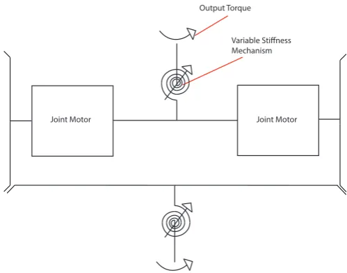
1.1 Simplified 2D representation of the Differential Drive including its

Joint Motors and the Variable Stiffness Mechanism (VSM). . . 2

2.1 Jack Spring Actuator with active and inactive coil regions and prin-ciple of changing stiffness by rotation of spindle. . . 4

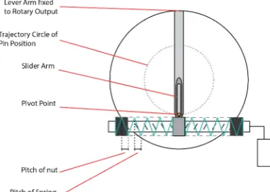
2.2 Principle of Lever Arm Mechanism . . . 4

2.3 Principle of VS Joint: Roller in equilibrium position with zero stiff-ness on the left hand side. Actuator Force F_A has to be applied to increase the stiffness by pretensioning the springs. On the right of the figure the joint is deflected byϕ. . . 5

2.4 Principle of FSJ: a) shows the FSJ in equilibrium position and stiff-ness preset φ0=0. The Springs are attached to the camdisks, can move in horizontal direction however. In b) the camdisks were ro-tated respectively to each other byφ_{sti f f} and the spring is expanded, so that the joint is in a stiff state. A deflection of the joint occurs when the rollers are moved out of their equilibrium position byϕin c) with an arbitrary stiffness preset ofφ1. . . 5

2.5 Adaptation of the ’Jack Spring’ towards use in the Differential Drive. 8 2.6 Eq. Position of Jack Spring in DD . . . 8

2.7 Deflection of Jack Spring in DD. . . 9

2.8 Adaptation of the Pretension Mechanism of ’DLR’ towards use in the Differential Drive. . . 9

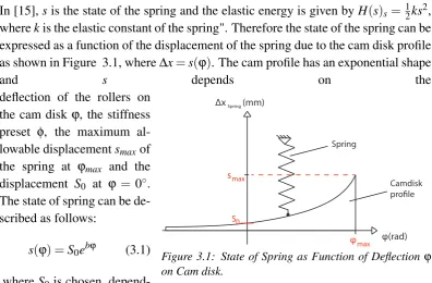
3.1 State of Spring as Function of Deflectionϕon Cam disk. . . 11

3.2 Different Spring Setups . . . 13

3.3 Torque-Deflection Plot for Different Spring Setups . . . 14

3.4 Deflection Range . . . 14

3.5 Force representation of the VSM mechanism. . . 15

3.6 Output Stiffness for different stiffness presets, starting withφ=0◦, so very compliant and ending with a stiff preset ofφ=20◦ . . . 16

(6)

4.1 Overview of Design of Variable Stiffness Mechanism . . . 25

4.2 More Detailed View of Design . . . 26

4.3 Exact Measurements of the Spring Space for Extreme Cases. . . 26

4.4 Variable Stiffness Joint including Motor, Gear and Clutch System. . 27

4.5 Labeled Section View of Variable Stiffness Joint in a) and the fric-tion clutch integrated into the Variable Stiffness Joint in b) . . . 28

5.1 SOLIDWORKS Model of Test Setup . . . 31

5.2 Deflection vs Output Torque for Springs used in Test Setup . . . 32

5.3 Fully Assembled Test Setup with F/T Sensor(right) and Magnetic Encoder(left). . . 33

5.4 Deflection vs Output Torque obtained by testing . . . 34

6.1 Compensated Deflection vs Output Torque Plot. The expected plots are deplicted in black colour. . . 36

A.1 Torque-Deflection MATLAB file for different Spring Setups, Page 1. 40 A.2 Torque-Deflection MATLAB file for different Spring Setups, Page 2. 41 A.3 Torque-Deflection MATLAB file for different Spring Setups, Page 3. 41 A.4 Zoom into fig.3.4:Output torque at a deflection of 25◦ _{. . . 41}

A.5 Plots of force approach and approach based on [15]. Plotted with a deflection range ofϕ= [−25◦25◦]andφ=0◦. τ10 andτcup is the torque produced by the springs on the upper cam profile. τ20 and τcdownis the torque produced by the springs on the lower cam profile. 42 A.6 Torque-Deflection MATLAB file for fundamental approach com-parison, Page 1. . . 42

A.7 Torque-Deflection MATLAB file for fundamental approach com-parison, Page 2. . . 43

A.8 Torque-Deflection MATLAB file for fundamental approach com-parison, Page 3. . . 43

A.9 Setup for the measurement of the Spring constantkincluding Newton-meter, weights(below) and scale. . . 44

A.10 Plot of Measured Spring Deflection vs Measured Force. The Data was evaluated using Matlab Curve Fitting withF=kxand resulted ink=0.7401[N/mm]. . . 44

B.1 Characteristic data of TQ Drive ILM25x08. . . 45

B.2 Characteristic Data of TQ Drive ILM38x06. . . 46

B.3 Characteristic Data of TQ Drive ILM38x12. . . 46

(7)

List of Tables

2.1 Evaluation of different VS-Mechanisms based on compactness and

robustness. . . 6

3.1 Values for input torqueτin and gear ratior withη=0.85 . . . 19

3.2 Values for input torqueτin and gear ratior withη=0.3 . . . 19

3.3 Values for gear ratior withη=0.85 divided byrHD . . . 20

3.4 Values for gear ratior withη=0.3 divided byrHD . . . 20

3.5 Gear ratiorbased onτnomin andτavg for additional motor models . . 20

3.6 Possible Arrangements of Motor. Upper horizontal column displays the placement of the motor in radial or axial position to the VS-mechanism. left Vertical row displays the shaft alignment of the VS-Mechanism as either parallel or perpendicular. . . 21

3.7 Possible gear and non-back-drivable element addition to previous motor arrangements. . . 22

(8)

(9)

Acknowledgments

First of all I would like to thank my supervisors Matteo Fumagalli and Raffaella Carloni for their support and advise throughout the course of my Bachelors Project. Special thanks go to Éamon Barrett, who helped me with his expertise and was always available to have a vivid discussion with. I consider him to be my second daily supervisor.

(10)

(11)

Abstract

In this study a variable stiffness mechanism with high torque output characteristics was developed for a differential drive. In doing so, different existing mechanisms and their underlying principles were investigated to elaborate further on a chosen design implementation. Based on this choice, the principle is modelled and realized according to the requirements imposed by the differential drive. Finally, validation of the model is achieved by tests of a simplified prototype.

(12)

(13)

Chapter 1 Introduction

The performance of robotic arms has been improving over the past years signifi-cantly. A broader performance necessity has become indispensable due to the adap-tation of robotic systems into subjects like medical application and manufacturing processes. Main objectives as a result of this adaptation and hence a closer human-robot interaction gives rise to criteria, like ’Interaction Safety’ or ’Shock Robust-ness’, as stated in [1]. On top of that autonomous robotics are generally in need of better physical interaction to avoid damage and manage tasks in an efficient and more adaptable manner. These criteria and demands paved the path towards an in-novation of Variable Stiffness Actuators (VSA), which can adjust the compliance of a joint based on which task it has to perform.

(14)

[image:14.595.160.410.106.302.2]

Joint Motor Joint Motor Variable Stiffness Mechanism Output Torque

Figure 1.1: Simplified 2D representation of the Differential Drive including its Joint Motors and the Variable Stiffness Mechanism (VSM).

(15)

Chapter 2 Evaluation of Variable Stiffness

Concepts

In Variable Stiffness Actuators a compliance adaptation and the control of equilib-rium position is achieved by two motors. Variable stiffness mechanisms rely on three elementary principles to achieve a compliance adaptation according to [4], which alter the compliance based on ’Changing Transmission between Load and Spring’, the ’Physical Properties of the Spring’ and ’Spring Preload’.

In this chapter different mechanisms of each principle are evaluated according to their applicability to the differential drive. Requirements for the High-Torque VSM, like a maximum Output Torque ofτmax =100[Nm]and dimensional restrictions of

100x130[mm](length and diameter of a cylinder, where the mechanism has to fit in) are the prime focus for this evaluation and form the goal of the research.

2.1 Compliant Joints

(16)

2.1.1 ’Physical Properties of a Spring’

Figure 2.1: Jack Spring Actuator with active and inactive coil regions and principle of changing stiffness by rotation of spindle.

Jack Spring Actuator

The principle of the ’Jack Spring’ Actuator [5] is to vary the effective length of a helical spring by adding or subtracting its coils. To do so, a rotating shaft divides the spring into active and inactive coil regions and thereby adjusts the spring force

F_s(ref. fig. 2.1).

Leaf spring Mechanism

The ’Variable Stiffness Joint using Leaf Springs’ [6] is another example of a varia-tion of effective length of a spring to manipulate the stiffness and is a post-design of the ’Mechanical Impedance Adjuster’ [7]. Instead of a common helical spring the joint implements four leaf springs. The stiffness of the leaf springs is adjusted by rollers, which can be considered pivot points moving on the leaf spring connected to the Output link.

2.1.2 ’Changing Transmission between Load and Spring’

Lever Arm Mechanism

Actuators like the vsaUT-II [8], mVSA-UT [9], AwAS [10] and AwAS-II [11]

real-Figure 2.2: Principle of Lever Arm Mechanism

[image:16.595.179.406.118.232.2]

(17)

2.1. Compliant Joints 5

2.1.3 ’Spring Preload’

Pretension Mechanism

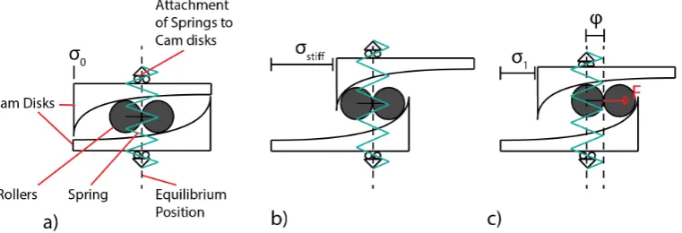
[image:17.595.118.499.528.658.2]

Adjusting the pretension of a spring by nonlinear profile manipulation is a typical example of ’Spring Preload’ and is adopted by the ’VS-Joint’ [12], the ’MACCEPA 2.0’ [13] and the ’Floating Spring Joint (FSJ)’ [14]. In fig. 2.3 the nonlinear profile of the spring of the ’VS-Joint’ can be seen together with the spring attached to a roller. In order to change the stiffness the spring is compressed

Figure 2.3: Principle of VS Joint: Roller in equilibrium position with zero stiffness on the left hand side. Actu-ator Force FAhas to be applied to increase the stiffness

by pretensioning the springs. On the right of the figure the joint is deflected byϕ.

by actuator forceFA, such that

the applied torque has to be bigger to move the roller up the cam profile, when increasing stiffness. The ’MACCEPA 2.0’ follows a similar approach, but makes use of a wire instead of rollers. The ’FSJ’ is based on a similar principle illustrated in fig. 2.4. Here one spring is at-tached to two cam profiles with exponential shape, which press onto a pair of rollers. Deflec-tion of the rollers, results in an

expansion of the springs, because the rollers move up one of the two profiles. The compliance can be adjusted by actuating the cam profiles with respect to each other in opposite direction such that the spring is extended and more force is required to excite the rollers.

Figure 2.4: Principle of FSJ: a) shows the FSJ in equilibrium position and stiffness preset

φ0=0. The Springs are attached to the camdisks, can move in horizontal direction

how-ever. In b) the camdisks were rotated respectively to each other byφsti f f and the spring is

expanded, so that the joint is in a stiff state. A deflection of the joint occurs when the rollers are moved out of their equilibrium position byϕin c) with an arbitrary stiffness preset of

(18)

2.2 Preliminary Evaluation

In this section advantages and disadvantages of each variable stiffness concept are discussed and evaluated according to the core requirements mentioned in the begin-ning of this chapter.

In all mechanisms the offset of compactness can be redirected to the size of the elastic element. This is because the spring element has to be able to produce a max-imum deformation that resembles a total torque of 100[Nm].However, the ’Preten-sion Mechanism’ of the ’MACCEPA 2.0’ is not compact due to the pulley system. In the ’Leaf Spring Mechanism’, the radius of the leaf springs was set to 40[mm] for the sake of space for housing or connections of the joint motors of the Dif-ferential Drive. The resulting calculation showed that for this leaf spring length and the defined output torque, the width of the leaf spring has a minimum value of

b=29.63 [mm] (A.1), which has a negative influence on the compactness of this mechanism (see tab.2.1). The remaining principles, the ’Jack Spring’, the ’Lever Arm Mechanism’ and the ’Pretension Mechanism (VSJ,FSJ)’ are evaluated based on the possible sizes of their springs. The ’VS-Joint’ employs three springs, the ’FSJ’ one big spring, the ’Jack Spring Actuator’ one spring and the ’Lever Arm Mechanism’ usually two. The ’Pretension Mechanism (VSJ,FSJ)’ seems to be the most promising about the adaptation of multiple springs and usage of conventional springs, which influence the robustness and compactness positively (ref. 2.1). An-other advantage is provided by its progressive torque deflection behavior, achieving high torques with high deflections.

The second factor, that needs to be evaluated is the torque requirement. A high output torque of the ’Jack spring’ Mechanism and Preload Mechanism (MACCEPA 2.0) is unlikely or at the cost of compactness, because they implement only one spring. Next a closer look is taken at the ’Lever Arm Mechanism’. A FEM-Analysis for stresses acting on the pivot pin of the ’mVSA-UT’ (shown in [9]) leads to doubt that the pivot in the lever arm mechanism can withstand high torques. However simple calculations were made in section A.2, that confute this.

Pretension Mech-anism (MAC-CEPA 2.0) Leaf Spring Mecha-nism Jack Spring Actuator Lever Arm Mecha-nism Pretension Mech-anism (VSJ,FSJ)

Compact - - +/- +/- +

Robust - +/- - +/- +

(19)

2.2. Preliminary Evaluation 7

(20)

2.3 Possible Implementation and Choice of Design

A tradeoff between the various mechanism specified previously was made to com-pare the possible implementation into the differential drive of two working prin-ciples. The ’Jack Spring Actuator’ and Pretension Mechanism were chosen to be analyzed further.

Figure 2.5: Adaptation of the ’Jack Spring’ towards use in the Differential Drive.

[image:20.595.86.277.466.602.2]

Fig. 2.5 depicts the ’Jack Spring’ integrated into the DD. In this particular design two springs are connected to the output and the active and passive coil regions are

Figure 2.6: Eq. Position of Jack Spring in DD

(21)

2.3. Possible Implementation and Choice of Design 9

Preload’ mechanisms.

The chosen alternative to the ’Jack Spring’ implementation is illustrated in fig. 2.8 and is founded on the ’VS-Joint’ and ’FSJ’ mechanisms. The rigidly connected cam profiles are located in the middle of the two joint motors. This design is

Figure 2.7: Deflection of Jack Spring in DD.

comparable to an inverse of the ’FSJ’ principle. However instead of having a hollow spring in the middle of the design the cam profiles are connected via shafts to the joint motors. The thought be-hind this is that conventional springs can be used instead of one custom made spring with a high spring constant and it is presumed that less

space is consumed by employing a rigid connection through the middle of the de-sign. Additionally the springs are connected to rollers on one side, which is similar to the ’VS-Joint’ and to rotating cups on the other side. This is contrary to the ’FSJ’ where the spring is attached to both cam profiles. The function of the rotating cups is to adjust the relative position of the rollers on the cam profiles to change the stiff-ness. Hence the stiffness motor rotates the cups against each other. The problems of this design mainly focus

Figure 2.8: Adaptation of the Pretension Mechanism of ’DLR’ towards use in the Differen-tial Drive.

(22)

element since it has to cope with the high torque. The ’Jack Spring’ actuator uses two springs as well as the alternative design. The roller-base and orientation of the springs in the shaft direction leaves more space to make use of bigger or multiple springs in the preload design.

(23)

Chapter 3 Modelling

3.1 Analysis of Variable Stiffness Mechanism

The chosen mechanism has to fulfill the requirements of 100Nm Output Torque, which is targeted by analyzing the variable Stiffness Mechanism in depth. Initially the output torque for different spring arrangements was calculated as in [15] and is subsequently checked by a more force approach.

3.1.1 Torque-Deflection Characteristics

In [15],sis the state of the spring and the elastic energy is given byH(s)s = 1₂ks2,

wherekis the elastic constant of the spring". Therefore the state of the spring can be expressed as a function of the displacement of the spring due to the cam disk profile as shown in Figure 3.1, where∆x=s(ϕ). The cam profile has an exponential shape

and s depends on the

φ(rad) Δx (mm)Spring

φ_max s

Camdisk profile

S₀

Spring

[image:23.595.114.511.446.706.2]

max

Figure 3.1: State of Spring as Function of Deflectionϕ

on Cam disk.

deflection of the rollers on the cam disk ϕ, the stiffness

preset φ, the maximum

al-lowable displacements_maxof the spring at ϕmax and the

displacement S0 at ϕ = 0◦.

The state of spring can be de-scribed as follows:

s(ϕ) =S₀ebϕ (3.1)

,whereS0 is chosen,

depend-ing on how sensitive the VSM should be and should not exceedϕmax of course.The

(24)

equa-tion, i.e. :

b= ln(

smax S0 )

ϕmax ,

where s_max=l_f−l_s (3.2)

The maximum displacement can be calculated by subtracting the solid length ls

from the free lengthlf of the chosen spring.

Next the Output torque has to be defined by making use of the state of the spring. From [15] it can be obtained that the ForceF at the Output Port can be described as F = −BT₍_q_,_r₎∂He

∂s (s). Noting that He(s) is the elastic energy of the

compli-ant element andB(q,r)is the sub-matrix defining "the relation between the rate of change of the output positionrand the rate of change of the statesof the elastic ele-ments" [15]. The latter can be described asB(q,r):=∂λ

∂r(q,r). According to Visser

λ:(q,r)7→s, so thatB(q,r):=∂_∂s_r. This can be inserted into the Force equation and finally eq. 3.3 can be obtained.

F=−∂s

∂r

∂He

∂s (s) (3.3)

The state of the springsdefined earlier however is expressed by the Output deflec-tionϕin radians and not in output positionr. Therefore ϕ= _rr_c, withrc being the

radius of the cam disk, has to be substituted into the displacement equation, such thats(r) =S₀ebrcr . Additionally eq. 3.3 should be defined as a output torque of a

spring on a cam disk by multiplying with the radius of the cam diskr_c. Accordingly eq. 3.3 is adapted andH(s)s ands(r)are inserted respectively, resulting in eq. 3.5

below.

rcF =τcam=−rc∂s

∂r

∂He

∂s (s) =−rc

∂s

∂rks (3.4)

=−krcb

r_cS

2 0e2b

r

rc ₌₋_kbS2₀_e2brcr (3.5)

Resubstituting ofϕ= _rr

c results in:

τcam(ϕ) =−kbS20e2bϕ (3.6)

Last but not least the output torque is also affected by the stiffness preset which is set by the stiffness motor and changes the apparent output stiffness. In order to change the Stiffness the motor has to move the position of the springs on the cam disks relative to each other as shown in figure 2.8 byφ. The resulting Output torque

is shown below:

(25)

3.1. Analysis of Variable Stiffness Mechanism 13

3.1.2 Torque-Deflection Plots

To realize the target of 100Nmoutput torque different spring setups and deflection ranges have been investigated. When plotting the torque-deflection it is important to sum up the output torques of the opposing cam-mechanisms to get the total output-torqueτext as in eq. 3.10.

τ_cam₍_up₎(ϕ,φ) =kbS₀2e2b(ϕ+φ) (3.8)

τ_cam₍_down₎(ϕ,φ) =−kbS2₀e2b(−ϕ+φ) (3.9)

τext=τcamup+τcamdown (3.10)

Consequently the springs and their alignment in the mechanism have to be cho-sen. For this setup Die-Springs were used, because they can handle heavy duty (see [23]) and thus have a higher spring constant k, compared to common com-pression springs, with the same dimensions. The springs setups used for the first torque-deflection plot are a single Die-Spring and four Die-Springs in parallel con-nected to the rollers on the upper and lower cam profiles. The implementation of four springs is motivated by the possible adaptation of multiple springs as discussed in section 2.2 to achieve a higher output torque. To stay within the specified limits of 100mmlength, the springs should not exceed a free length oflf ≤40mm.

Addition-ally the single Spring should have a diameter that is large enough to leave enough space for a shaft passing through. The four springs on contrary are positioned

Camdisk Profile

40 mm

Spring x4 Shaft

Figure 3.2: Different Spring Setups

around the shaft. Thus it is of impor-tance that they fit within the specifi-cations of 130mm in diameter of the mechanism. To accomplish the latter, the cam disks have been given a radius of r_c =40mm and the diameter of the parallel arranged springs has to fit in between the cam profile and the shaft as shown in 3.2. A rough estimate

provides that the diameter of the parallel springs has to be smaller than 20mm. Next the spring components are chosen depending on the requirement to fit into the VSM. Eventually the spring [24] was chosen as the single spring setup with

k=144.45N/mmandl_f =38.1mm. The spring for the parallel setup is [25] with a spring constant ofk=47.62N/mm, the same free length as for the single setup and a outer diameter ofD0=14.808. Since there are four springs in parallel the

(26)

subsection 3.1.1 for each spring setup and eventually the total output-torque was calculated by making use of eq. 3.10. This can be seen in fig. 3.3. To review the entire calculation, the MATLAB file can be checked in APPENDIX A (A.1 - A.3).

−15 −10 −5 0 5 10 15

−200 −150 −100 −50 0 50 100 150 200

τ_ext(N m)

ϕ(deg)

Single Spring

[image:26.595.150.412.166.331.2]

Four Springs in Parallel

Figure 3.3: Torque-Deflection Plot for Different Spring Setups

In fig.3.3 each of the spring-setups have three subplots. This is because every plot was made with three different stiffness presets ofφ=0, 0.05 and 0.1[rad]. Ana-lyzing this first Torque-Deflection plot, it can be stated that due to a lower stiffness preset the total Output torque has a smaller total deflection, which is what would be expected. Besides, the total Output-Torque for the setup using multiple springs on each side is higher than the Output-Torque for the single spring setup. This has two main reasons. First of all the spring constant is higher and secondly each spring has

−50 0 50

−200 −150 −100 −50 0 50 100 150 200 τ_ext ϕ

ϕ∈[−15 15◦_]

ϕ∈[−25 25◦_]

ϕ∈[−50 50◦_]

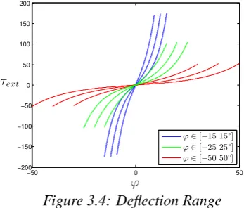
Figure 3.4: Deflection Range

a greater allowable displacement, be-cause each individual spring is more compliant than the single-spring setup. All in all, this plot encourages the choice for multiple spring-setup, also because if using a single spring with the same free lengthl_f, the diameter of the rod will become rather small, when try-ing to achieve the same Output-Torque amplitude.

In the following part, the analysis will focus on the Deflection-Range of the cam-profile to realize the required 100Nm. The Deflection-Range has an impact on the torque amplitude due to the fact that is also scales thebparameter of the state of the springs(ref. eq.3.2). Such that each state of spring for a chosen deflection had to be recalculated before plotting, includ-ing the sprinclud-ing characteristics for the parallel sprinclud-ing-setup. The chosen ranges are depicted in fig.3.4 and also here different Stiffness-Presets by changingφ to 20%

[image:26.595.90.264.476.624.2]

(27)

3.1. Analysis of Variable Stiffness Mechanism 15

plots in APPENDIX A fig.A.4 reveals that atϕ=25◦_{the Output torque is 105}_.₃_Nm_.

Concluding it is to mention, that the deflection range ofϕ= [−25 25◦]is closest to the target Output-Torque. Thus this range is applied to the design of the mechanism together with four springs in parallel on each side.

3.1.3 Force Approach

The former approach to calculate the Output torque depending on deflectionϕand stiffness preset φ is based on a method given by [15]. To confirm this method a more fundamental approach has been investigated, based on a force model of the mechanism. When the spring is compressed, due to movement of the rollers on the cam-profile, it creates a forceF_s acting on the cam profile, as illustrated in fig.??.

The resulting Forces acting on the exponential profile areF_N acting normal to the profile andF10, which is the output force. For the sake of retrieving the total output

Force Ftot, the output force F10 has to be evaluated in every point x0 on the

2D-profile and summed up with the output force on the opposing 2D-profileF20. Lastly the

total output force will be converted into torqueτext by multiplying withrc=40mm.

x ∆x_Spring m 1 m 1

F_N _S

10

F

a

Figure 3.5: Force representation of the VSM mechanism.

Primarily the displacement of the spring has to be rewritten to be depen-dent on x and not on ϕ, by inserting

ϕ=x/rc. So equation 3.1 transforms

to

s(x) =S₀ercbx₌3_.1e3.284640 x (3.11)

Based on the Force of the spring Fs =

ks(x)and the angleαall other forces in

the model can be expressed as follows:

FN = 1

cos(α)Fs (3.12)

F₁₀ =sin(α)F_N (3.13)

At this moment all parameters are defined except angleα, which can be calculated

by making use of the slopemofs. The slopemis equal to the derivative ofsinx0

(3.14).

m=tan(α) = ∂s(x0)

∂x (3.14)

α=tan−1(∂s(x0)

(28)

The plots and MATLAB-file can be reviewed in APPENDIX A (fig.A.5 and fig.A.6-A.8). Fig.A.5 illustrates that the force approach is indeed identical to the former method. However this can also be proofed in a more simple manner. Inserting equation 3.13 into equation 3.12 and eventually substitutingtan(α), leads to

F₁₀

sinα =

1

cos(α)Fs (3.16)

F10= sin(α)

cos(α)Fs=tan(α)Fs=mFs=

∂s(x₀)

∂x Fs (3.17)

The result is identical to eq.3.3.

3.1.4 Apparent Output Stiffness

A plot was made of the output-stiffness against the output-torque, calculated in the previous sections. As in [15], the apparent output stiffnessK can be described as the ratio of the infinitesimal change of the actuator output force∂F, as a result of an infinitesimal displacement of the actuator output position∂r. In the case of the cam mechanism this can be reformulated toK = ∂τcam

∂ϕ . The result of this rather simple

calculation can be viewed in fig.3.6.

0 20 40 60 80 100

0 50 100 150 200 250 300 350

Output Stiffness (Nm/rad)

Output Torque (Nm) Output Stiffness for Different Stiffness Presets

φ= 0◦

φ= 5◦ φ= 10◦ φ= 15◦

[image:28.595.194.373.447.588.2]

φ= 20◦

Figure 3.6: Output Stiffness for different stiffness presets, starting with φ=0◦_{, so very}

compliant and ending with a stiff preset ofφ=20◦

The figure confirms that the stiffness presetϕis included correctly in the output-torque equation, since for a compliant setting ofφ=0◦_{the mechanism is at its most}

compliant with aboutK=20Nm/rad at low torque-output. Vice versa the highest Stiffness at low torque-output of K =195Nm/rad is achieved for φ =20◦_{. The}

highest Stiffness can be achieved however with every stiffness preset ofφ, because

(29)

3.2. Motoranalysis 17

3.2 Motoranalysis

This section emphasises on Power-, Volume- and Dynamic Analysis to gain insight into the requirements of the motor. The specifications obtained by the different analysis serve as a feasibility study for the motor including gearbox to fit into the design and comply with the given requirements of 100Nmoutput torque.

3.2.1 PowerAnalysis

To identify the parameters necessary to make a Power-analysis other variable stiff-ness actuators, their Nominal Stiffstiff-ness Variation Times and Nominal Speed charac-teristics have been investigated. The vsaUT-II provides a Nominal Stiffness Varia-tion Time of 0.6[s]with a Nominal Speed ofπ[rad/s],while the FSJ provides values of 0.33[s]and 8.51[rad/s]respectively.

The Power will be determined by using the average torque τavg[Nm] and angular

velocity(Speed)ω_avg[rad/s], as described in:

Pavg=ωavg∗τavg (3.18)

The average torque (τavg) can be obtained by taking the average of the maximum

and minimum torque required to get a completely stiff and compliant setting of the VSM, i.e.:

τavg =τmax+τmin

2 (3.19)

In order to change the Stiffness, both of the opposing spring mechanisms have to be either compressed or expanded at the same time. This means that in order to get the maximum torque at an angle ofσmax=25◦for both cam disks, the maximum torque

obtained throughτ_camdisk(σmax)has to be multiplied by 2. The minimum torque is

computed the in the same manner except thatσmin=0.1◦. So by calculatingτcamdisk

with respect toσwe get:

τ_camdisk= ds

dσks≈5999.5e

6.6σ _(3.20)

Insertingσ_max,σ_min and multiplying by 2 results in:

τmax≈209.135[Nm],atσmax (3.21)

(30)

And by making use of Equation (3.19) we getτavg≈110.636[Nm].

The average angular velocity can be calculated by the following equation:

ω_avg=2σavg

tnom (3.23)

wheretnomis the Nominal Stiffness Variation Time chosen for this VSA andσavg is

the nominal angle, which can be calculated by usingτavg as follows:

τavg

2 ≈5999.5e

6.6σavg _(3.24)

σavg≈

ln(₁₁₉₉₉τavgnom_.₁)

6.6 (3.25)

and thus the nominal angle ofσavg≈0.3391[rad].

The Nominal Stiffness Variation Time was chosen to be tnom = 1[s], despite the

Stiffness Variation Times of investigated VSAs, compensating for the high nominal torque in eq. (3.19). The necessity of this measure evolves from the fact that the power-consumption has to be kept low to allow a usage of small motors, which still fit into the design. Based on the calculated values and equation 3.23, the average an-gular velocity isωavg≈0.678[rad/s]. Equation 3.18 then givesPavg≈75.039[W].

3.2.2 Transmission Analysis

The ‘Robotic Optimized Servodrive’ series (TQ Robodrive) was chosen to be used, since the dimensions have to be kept compact. The TQ Robodrive enables the latter by offering the possibility to design customized housings for the chosen motor. Different types of the "Robodrive" permit different input torques τ_in, which will be obtained from the figures in the Appendix by calculating the current amplitude

Iin. The current amplitude can be calculated by taking the rated voltage of 24V

and 48V and the previously determined Power Pavg. Taking Pavg =IinVin results

in Iin =3.126 A and Iin =1.563 A for Vin = 24,48V respectively. Due to these

values for I_in values for the input torques τin can be obtained from the figures in

the APPENDIX B and are depicted in Tab. 3.1. The values for the ‘ILM 25x08’ and ‘ILM 38x06’ by ’TQ-Group’ are about the same, thus there is only one row in Tab. 3.1 for both.

To continue with the Volume Analysis, it is necessary to know the size of the gear, that has to be combined with the motor in order to get the desired average torque ofτavg≈110.636[Nm]. The size of the gear can be estimated by calculation of the

(31)

efficiency of the gearboxη, as shown in eq. (3.26).

r=τnom

ητ_in (3.26)

The gear mechanism has to be non-back-drivable, such that the stiffness motor does not have to supply constant torque and subsequently the energy efficiency of the VSA is increased. To ensure that the gear ratio will not increase significantly due to inefficiency caused by the use of for example worm gearboxes, hypoid gears can be used as non-back-drivable elements. The efficiencyη of worm gears can be as

low asη=0.3 %, while the efficiency of hypoid gears is about 0.85≤η≤0.96 %

as shown in [16]. To get a worst case estimation, the lowest efficiency ofη=0.85

is taken and results are depicted in Tab. 3.1 together with the input torquesτ_in.

ILM 25x08/ILM 38x06 ILM 38x12 ILM50x08

τin[Nm] r τin [Nm] r τin[Nm] r

24 V 0.051 2552.16 0.11 1183.27 0.25 520.64 48 V 0.024 5423.33 0.055 2366.54 0.125 1041.29

Table 3.1: Values for input torqueτinand gear ratio r withη=0.85

Tab. 3.1 already points out that the gear ratios are at a level where the implemen-tation of a single stage gear becomes obsolete. Therefore high efficient Harmonic Drives could be implemented together with a hypoid gear. If using a worm-gearbox the mechanism would probably consist of two gear stages and the worm gearbox to achieve the necessary gear ratio. Values for the gear ratio when implementing a worm gear are shown in table 3.2.

ILM 25x08/ILM 38x06 ILM 38x12 ILM50x08

τin[Nm] r τin [Nm] r τin[Nm] r

24 V 0.051 7231.11 0.11 3352.61 0.25 1475.15 48 V 0.024 15366.11 0.055 6705.21 0.125 2950.29

Table 3.2: Values for input torqueτinand gear ratio r withη=0.3

(32)

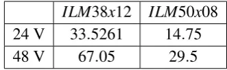
ILM38x12 ILM50x08 24 V 11.83 5.21

[image:32.595.199.367.103.154.2]

48 V 23.67 10.41

Table 3.3: Values for gear ratio r withη=0.85divided by rHD

ILM38x12 ILM50x08

24 V 33.5261 14.75

[image:32.595.199.365.197.248.2]

48 V 67.05 29.5

Table 3.4: Values for gear ratio r withη=0.3divided by rHD

The left over gear ratios in tab. 3.3 can be achieved with the harmonic drive and a hypoid gear, whereas the gear ratios from tab. 3.4 probably need a second gear stage or an extra harmonic drive before the worm gear stage, but this still depends on the efficiency of the chosen worm-gear.

An alternative to a bulky gear mechanism due to the use of a non-back-drivable gear element was developed by replacing the non-back-drivable element by clutches. If the gear mechanism is smaller a bigger motor with higher input torque can be used and the implementation of a single gear stage becomes arguable. On top of that the clutches do not have a drawback caused by lower efficiency which means that in a setup without non-back-drivable gear element the efficiency can be set toη≈1. The "ILM70x10" and "ILM-85x13" are the thin versions of the big "Robodrive" have nominal input torques ofτnomin =0.74[Nm]and 1.43[Nm]at a nominal power

consumption ofP_nom=270[W]and 450[W]respectively according to [26]. Impor-tant to mention here is that the input torque at lower power consumption, like 75[W] is not significantly higher than in the previous calculations. However these motors have a broader performance range and therefore enable higher input torques, at cost of larger power consumption. Using the former calculation of gear ratio with ef-ficiencyη=1 and the nominal input torques of the bigger motors, results in table 3.5.

ILM70x10 ILM85x13

r 149.51 77.37

Table 3.5: Gear ratio r based onτnominandτavgfor additional motor models

These gear ratios can definitely be handled by a single gear stage like the "25-CSD-2A Harmonic Drive" (ref. [27]) with a gear ratio ofr=160. Another advantage of the smaller gear ratios in tab.3.5 and higher power consumption is that the angular input velocityωinwill be greater and the nominal Speed and Stiffness variation time

(33)

3.2.3 Volume Analysis

Figure 3.7: 2D-View of the Assembly without Motor, all dimensions in mm.

Fig.3.7 shows a 2D-Representation of the mechanism in this report. The VS-Mechanism depicted already gives a preview to the Design chapter and will help with the volume analysis. The goal of this section is to find a placement of the motor and gear such that the entire module does not exceed the dimensional limits of 130mm in diameter and 150mm in length. The Volume Analysis starts with a possible arrangements of the motor with respect to the variable stiffness mechanism, shown in tab. 3.6.

Radial Axial

⊥

k

Table 3.6: Possible Arrangements of Motor. Upper horizontal column displays the place-ment of the motor in radial or axial position to the VS-mechanism. left Vertical row displays the shaft alignment of the VS-Mechanism as either parallel or perpendicular.

(34)

alignment of the motor shaft to the VS-shaft and in axial or radial placement of the motor to the VS-mechanism. From this simple diagram the different possibilities in gear combinations can be derived and evaluated.

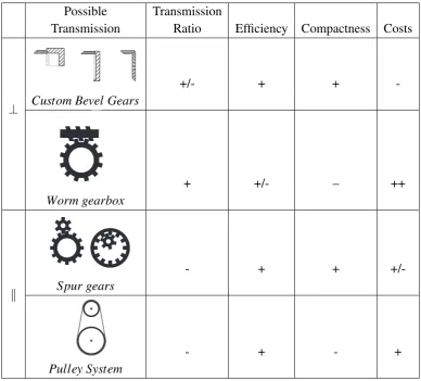
Possible Transmission

Transmission Ratio Efficiency Compactness Costs

⊥

+/- + +

-Custom Bevel Gears

+ +/- – ++

Worm gearbox

k

- + +

+/-Spur gears

- + - +

[image:34.595.89.478.162.513.2]

Pulley System

Table 3.7: Possible gear and non-back-drivable element addition to previous motor ar-rangements.

For the perpendicular shaft alignment of stiffness mechanism and motor, custom bevel gears or a worm gearbox can be used, whereas for parallel alignment spur gears or a pulley system can be chosen referring to tab. 3.7. As shown in previ-ous chapter when relying on a small motor at least one other gear stage in terms of a harmonic drive has to be implemented together with each of the gears in the table above. Whilst the perpendicular arrangements already enable non-back-drive-ability, the gears for the parallel shaft alignments have to be decoupled by using clutch mechanisms.

(35)

evaluated further by the manufacturer. Especially hypoid gears are known for their high transmission ratios. As explained earlier in this section the efficiency of bevel gears is rather promising compared to worm gearboxes because the friction compo-nent -which makes worm gears non-back drivable- is higher at lower speeds. Due to the small size of the worm the allowable transmission ratio offers a promising range of upper limit values. The worm gear is available as complete gearbox modules; lowering the costs but affecting the compactness negatively. The gears depicted in 3.7 for a parallel arrangement of motor and mechanism shaft have similar charac-teristics concerning the transmission ratio and efficiency on one hand. Comparing the compactness however the pulley system has to be placed further apart and thus occupies more space in the mechanism. The Spur gear would probably have to be custom made to fit into the requirements of the mechanism affecting the costs. It is however less expensive than the custom made bevel gear.

3.2.4 Choice of Motor and Gear Combination

Concluding the motor analysis, a comparison is made between the transmission for different motor types as shown in subsection 3.2.2 and available gear combinations evaluated in subsection 3.2.3. The smaller motor models (tab. 3.1) are in need of a higher transmission than the bigger robodrive models. Thus a perpendicular shaft alignment should be chosen according to tab. 3.7 since the bevel gear and worm gear offer greater transmission ratios. Furthermore the bevel gear would have to be made by a specialist in order to be non-back-drivable or a clutch has to be added. Thus the worm-gearbox should be used together with a harmonic drive for a small motor.

If using a bigger motor (tab. 3.5) a parallel shaft alignment can be chosen since the needed transmission ratios are smaller. Additionally the inner diameter of the bigger motor models is sufficiently large enough to make the mechanism shaft pass through and use a hollow spur gear, which is more compact than a pulley system or harmonic drive. If using a harmonic drive the gear stages can be reduced to a single gear stage and a clutch mechanism ensuring self locking of the mechanism.

(36)

(37)

Chapter 4 Design

The design chapter consists of two parts about the realization of the variable stiff-ness mechanism and of the Stiffstiff-ness Actuation relying on the decision made in section 3.2 respectively. The Drawings were done in ’SOLIDWORKS2012’. Spe-cial attention in the design of the VSA is paid to the dimensional requirements given as 100[mm]length and 130[mm]in diameter.

4.1 Variable Stiffness Mechanism

(a) Front View of Preload Mechanism with transparent Rotational Cups

(b) Side View of Preload Mechanism

Figure 4.1: Overview of Design of Variable Stiffness Mechanism

According to section 3.1 the compliant mechanism has to include four springs on each side of the cam-disks shown in fig. 3.2 and the exponential cam profile specified in equation 3.1 with the chosen spring and a deflection range of ϕ= [−25◦25◦]. Thus the state of spring on the profile should bes_cam(ϕ)≈3.1e3.2846ϕ

(38)

Rollers Roller-Base Shaft Linear Bushing Bushing Housing Rotating Cup Thin Section Bearings Camdisk Bearing Stop Guidance Bearing Spacer Low Head Shoulder Bolt

(a) Section View Front Plane

Springs Guidance

Adapter

Mechanical Stops

(b) Top View

Figure 4.2: More Detailed View of Design

100[mm]in length and 115.138[mm]as its maximum diameter.

All different components and their labels can be viewed in Section View 4.2a) and Top View 4.2 b). The main shaft has to be connected via Bearing Stops to the joint motors (ref fig. 2.8) on each side and is attached to the opposing cam disks in the middle. The specified cam profile has an offset of 6.5 [mm], because radius of the cam rollers, which are ball bearings ( [28]) in this case has to be taken into account. The rollers are mounted by ’Low Head Shoulder Bolts’ [29] to the roller-base. The roller-base and the rotating cup define the endpoints of the spring. At this point it has to be taken heed of that the length of the spring at minimum deflection can not exceedl_f−s_cam(ϕ_min)≈38.1−3.1e3.2846(−25₁₈₀pi)_≈₃₇_.₃₆₀₅_[_mm_]

and 38.1−12.995 = 25.105[mm]for maximum deflection, this is verified when taking a look at illustration 4.3. The real values differ by 0.0717337 [mm] and 0.0169578 [mm] for the roller in minimum and maximum position on the profile. This also proves that the offset given to the calculated shape of the profile is correct. The rotational cups have to rotate together with the roller-base considering that a

(a) Spring length for maxmal deflection of 25◦ _{(b) Spring length for minimal deflection of}₋₂₅◦

Figure 4.3: Exact Measurements of the Spring Space for Extreme Cases.

(39)

4.2. Motor and Gear Module 27

have been implemented. The so called guidance bearing is as well fixed with a shoulder bolt, via guidance adapters (yellow parts) to the roller-base. Additionally the roller-base should be centered around the shaft, which is achieved by a linear bushing [30] on each side. The linear bushing is attached through a housing to the roller-base. The rotational cups have to be supported on each side by Thin section bearings with bore diameter of 25[mm][31] and 90[mm][32] The small thin section bearings are supported on the other side by bearing stops, which can later on be connected to the differential drive. In this way the Springs are pressed together by the roller-base and the rotational cup.

4.2 Motor and Gear Module

At this stage it got obvious that it is impossible to fulfill the dimension require-ments, because the previously designed stiffness mechanism has already reached dimensional limitations that make the design of the motor within the given require-ments unfeasible. It could be argued that there is still space in the radial direction, but even with a small motor the gear system will be too bulky, which is proved in subsection 3.2.2. On these grounds the requirements were adapted to 150[mm]in length and still 130[mm]in diameter. The entire variable stiffness actuator is repre-sented in fig. 4.4. Its uttermost dimensions are 153.6[mm]in length and 135[mm]in diameter.

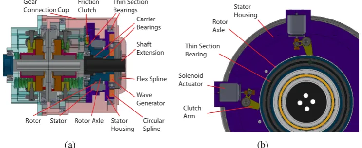
Figure 4.4: Variable Stiffness Joint including Motor, Gear and Clutch System.

(40)

’TQ-Robodrive ILM70x10’ is fixed to the right rotating cup via the Stator Housing whilst the Rotor has to be connected through the ’25-CSD-2A Harmonic Drive’ to the left rotating cup. The stator housing is also attached to the circular spline on the right side to hold the ’Harmonic Drive’ in position. The Rotor axle is attached to the input, also called wave generator of the HD and is rotationally supported by carrier bearings with bore diameter 20[mm] [33] and 17[mm][34]. In order to understand the drawing it should be noticed, that the shaft extension mounted to the main shaft of the mechanism still has to be attached to the differential drive, which is why the rotor housing and the HD are hollow. Last but not least the Output of the harmonic drive - the flex spline - is linked to the left rotating cup via the gear connection cup. The gear connection cup is stored by two thin section bearings with bore diameter 90[mm][32] and 110[mm][35].

Rotor Axle Shaft Extension Thin Section Bearings Gear Connection Cup Flex Spline Wave Generator Circular Spline

Rotor Stator Stator

[image:40.595.109.481.328.480.2]

Housing Carrier Bearings Friction Clutch (a) Solenoid Actuator Rotor Axle Clutch Arm Stator Housing Thin Section Bearing (b)

Figure 4.5: Labeled Section View of Variable Stiffness Joint in a) and the friction clutch integrated into the Variable Stiffness Joint in b)

Another thin section bearing( [36]) supports the rotor axle on the same position, where the friction clutch is located, as can be seen more detailed in fig. 4.5 b). The friction clutch is designed with a logarithmic profile and a contact angle of 8◦

(41)

4.3. Datasheet 29

4.3 Datasheet

Due to the broad range of variable stiffness actuators and their different fields of application, a VSA datasheet has been developed in [18], which can serve as a set-point for the comparison of the developed mechanism for postprocessing. The Design and Modelling chapters provide the input for said datasheet and the result can be seen below in tab. 4.1.

High Torque VSM-UT

Spring Preload

Operating Data

# (quantity) (unit) (value)

Mechanical

1 Continous Output Power [W] 67.488

2 Nominal Torque [Nm] 55.318

3 Nominal Speed [rad/s] 1.22

4 Nominal Stiffness with no load [s] 0.2779 5 Variation Time with nominal torque [s] 0.2779 6 Peak (Maximum) Torque [Nm] 105.3

7 Maximum Speed [rad/s]

-8 Maximum Stiffness [Nm/rad] 347 9 Minimum Stiffness [Nm/rad] 24 10 Maximum Elastic Energy [J] -11 Maximum Torque Hysteresis [◦_]

-12 _{Maximum Deflection} with max. stiffness [◦_]

-13 with min. stiffness [◦_] ₂₅

14 Active Rotation Angle [◦_]

-15 Angular Resolution Angle [◦_]

-16 Weight [kg]

-Electrical

17 Nominal Voltage [V] 48

18 Nominal Current [A] 5.625

19 Maximum Current [A] 35.417

0 20 40 60 80 100

0 50 100 150 200 250 300 350

Output Torque (Nm) Output Stiffness for Different Stiffness Presets

φ= 0◦ φ= 5◦

φ= 10◦

[image:41.595.114.534.221.565.2]

φ= 15◦ φ= 20◦

(42)

(43)

Chapter 5 Proof of Concept

Theoretically there is already a possible implementation with adapted requirements presented in the previous chapter. It is of importance however, that the theory of chapter 3.1 is validated by a proof of concept before purchasing rather expensive components like the ’TQ Robodrive’, the ’Harmonic Drive’ and the thin section bearings. Hence the adaptation of the design towards (rapid prototyping) usage of cheaper components and measurement equipment is the first part of this chapter. Later on the new design is tested accordingly.

[image:43.595.156.486.484.683.2]

5.1 Adaptation of Design/Rapid Prototyping

Figure 5.1: SOLIDWORKS Model of Test Setup

(44)

compliant springs, that are available in the RAM-group laboratory replace the Die Springs. The spring constant k had to be evaluated and was measured using a newton-meter and different weights. The Setup can be seen in Appendix A (fig.A.9) together with a plot of the measured Force vs Deflection (fig. A.10), resulting in a spring constant ofk=0.7401[N/mm].

Based on this Spring constant and the modeling of Output torque related to the state of spring explained in chapter 3.1 a Deflection vs Output torque plot for the test setup can be calculated. The spring used for the test setup has a free length of

lf ≈56[mm], whereas the calculations for the cam profile were based on a spring

withl_f =38.1[mm]. Regarding this aspect the state of spring has to be modified such that an initial compression of 56−38.1 [mm] is added. The results of the calculated Torque based on the state of springsare shown below in fig. 5.2.

−30 −20 −10 0 10 20 30

−4 −3 −2 −1 0 1 2 3 4

[image:44.595.143.413.335.552.2]

Output Deflection (deg)

Figure 5.2: Deflection vs Output Torque for Springs used in Test Setup

(45)

ten-5.2. Test and Results 33

sioned by adjusting the motor position on the base plate. One might notice that this test setup is back-drivable since no breaks are included in the model. One of the rotating cups was attached to the base plate together with the motor. This implies that the design is reversed for testing and the torque has to be applied to the main shaft instead of the rotating cups. Consequently the main shaft has to be

Figure 5.3: Fully Assembled Test Setup with F/T Sen-sor(right) and Magnetic Encoder(left).

kept in place by a bearing connected to the base plate (inside the orange connec-tor on the rightmost side of fig.5.1). To obtain the Out-put torque τ_out a force˜torque Sensor ’ATI mini 40’ was used and the deflection angle

ϕ was measured by a

mag-netic encoder ’AS5048A Ro-tary sensor’ shown in picture 5.3. Torque was applied by attaching a perspex bar to the

torque sensor. The frame parts, such as the base plate, the part aligning the encoder with the main shaft and the parts that hold the main shaft on the right hand-side were laser-cut. The main shafts inside of the VSA-mechanism attached to the cam pro-files were made out of aluminum by turning, because the linear bearing that centers the roller-base would impose friction if using plastic material. All other parts were 3D-printed. The data of the encoder was read by an ’Arduino Mega 2560’ con-nected to a USB-port and the force˜torque sensor by a Net Box concon-nected through Ethernet. Capturing and processing was done by a ’Real-Time-Workshop Simulink’ Model.

5.2 Test and Results

The goal of the testing is to show that the prototype behaves like expected or in other words that the plots of fig.5.2 are repeatable. Therefore the setup had to be tested for four different stiffness presets and the torque should be applied in a continual and non-disruptive manner. According to these criteria the measurements were carried out and resulted in the plots of hysteresis shown in fig. 5.4. Two hysteresis loops ranging from minimum to maximum possible deflection angle are plotted for each stiffness preset.

(46)

[image:46.595.97.460.239.535.2]

diagonal through the minimum and maximum values for deflection and torque will have a steeper slope for increasing stiffness presets - resulting in higher stiffnesses for higher stiffness presets. So in that concern the Prototype behaves like expected. Though the shape of each loop is not entirely smooth, the progressive shape of each loop is the same as in the expected plots. On top of that the maximum and minimum Output torque values seem to respond to the expected plots, except for the torque values of the green curve (φ=5◦_{), which overshoot by a small amount.}

Figure 5.4: Deflection vs Output Torque obtained by testing

Regarding the aspects in which the test setup did not perform as presumed it is clear that there are some issues with the minimum and maximum deflection angles compared to the calculated values. For the stiffest setting ofφ=15◦or the red curve in the figure 5.4 the range should be fromϕ=−10◦ to ϕ=10◦ and it actually is

ϕ≈[−8.8◦8.8◦]. Which is still reasonable regarding the friction in the test setup.

Forφ=0 and an assumed range of [−25◦₂₅◦_{], the measured deflections however}

range fromφ≈ −17.2◦_{to 17}_.₂◦_{. During the test of the prototype play and slip of}

(47)

Chapter 6 Discussion

The dimensions of the design realization of chapter 4 are not within the limits of the adapted requirements of 130[mm]in length and 150[mm]in diameter. However if integrated properly into the DD, a length of 150[mm] can probably be achieved when rearranging some components on the interface. In any case the requirements are already altered towards a rather large Variable Stiffness Joint compared with the models the VSM is based on (’VS-Jonit’ and ’FSJ’). A reason for this could be the necessary connection between the two joint motors of the differential drive, which is not a part of the existing VS models. A possible solution towards a more compact variable stiffness actuator could be to reconsider the implemented springs. In the fig. 4.1 it can be observed that there is some space lost next to the linear guidance on both sides of the rollerbase. This space can probably be used more efficiently if integrating more but shorter springs in a closed circle around the shaft. This could lead to a shorter VS-mechanism and would make room for the big motor and gear system. On the other hand the mechanism is quiet complex and redesigning will take some time, that could also be spend investigating on a new high torque vari-able stiffness actuator based on for example the lever arm mechanism. Contrarily, the progressive torque-deflection behavior of the adapted VS-principle is leading to benefits in the maximum torque characteristics for a broader range in stiffness settings compared to the lever arm mechanism.

Additional time has to be spend on the testing of the clutches, because only three out of the 10 tests of differently configured clutches were actually self locking in [17]. An alternative to this could be the use of a worm gearbox which would be feasible if the entire mechanism is more compact.

(48)

[image:48.595.97.457.208.495.2]

is still some deflection at hand. During the test these measurement errors were en-countered by trying to collect less data points at zero torque, which did not work out entirely. An attempt to make up for these errors by measuring the total shift in deflection for zero torque and zero stiffness preset and including it into the plot is made in fig. 6.1 below.

Figure 6.1: Compensated Deflection vs Output Torque Plot. The expected plots are deplicted in black colour.

For the zero stiffness preset half of the range (a factor 1.571) is taken as a gain for

(49)

Chapter 7 Conclusion and Future Work

7.1 Conclusion

The report presents a possible ’High-Torque VSM’ solution for the Differential Drive. Possible is the key word, because the VSM design would have to be adapted to fit into the DD and the components are expensive as well as not mainly off-shelf. The High-Torque task was fulfilled at the expense of a complex mechanism and design.

The Tests resulted in anticipated performance and validate the concept except for the deflection characteristics. The two hysteresis plots for each stiffness preset on top of each other show that the measurements are repeatable and the joint behaves in an adequate manner even though the tests were executed with a rapid prototype. Altogether this work emphasizes on the antagonistic aspects of the high torque and compactness requirements. Achievements of one and the other is still an obstacle, but not impossible.

7.2 Future Work

• Possible recalculation of Spring setup for a more compact actuator • Replacing roller (bearing plus shoulder bolt) by actual cam rollers • Adjusting Rotor Axle and Stator Housing to be reusable

• FEM ANALYSIS of the mechanism, especially shaft, which is the most likely component that needs checking (only try-out done in SOLIDWORKS and not part of report)

• Research on self-locking breaks and testing of proposed breaks

• Research on torsional spring between rotating supports to shift equilibrium

(50)

(51)

Appendix A

A.1 Calculation of Leaf Spring

According to [19] the maximum deflection of a leaf spring can be described as:

δmax =4Fl

3

Ebt3 (A.1)

WhereE is the modulus of elasticity taken as 180[GPa]for stainless steel [20],l

is the characteristic length of the spring, which was chosen to be 40[mm],F is the applied force of F = 100000₄₀ [Nmm_mm ] =2500N, bis the width andt is the thickness. Interesting in this calculation is the relation of width and thickness, when setting the maximum deflection toδ_max=10,15[mm].

For δmax=10[mm]: (A.2)

bt3=355.56[mm4] (A.3)

For δmax=15[mm]: (A.4)

bt3=237.04[mm4] (A.5)

Assuming that a maximum thickness of t =2[mm] the leaf spring would still be compliant without occurrence of permanent deformation, the width isb=44.44[mm] andb=29.63[mm]fordeltamax=10,15[mm]respectively.

A.2 Calculation of Pivot Point Dimension for Lever

Arm Mechanism

The shear force acting on the pivot pin can be calculated by the following equation from [21].

τUSS= 2F

(52)

In this equationτUSSis the ultimate shear stress,F the applied force anddthe

diam-eter of the pin, which we are interested in. The ultimate shear stress can be obtained by evaluating τUSS ≈0.75τUT S due to [22], with τUT S=860 [MPa]( [20]). The

torque-deflection plot of the ’vsaUT-II’ in [8], shows that for the smallest deflection the biggest Output torque is achieved. So it can be assumed that the pin is close to the Output. If the complete lever arm would be 10[cm], it is assumed that the distance between the Output and pin would be approximately 1[cm]to withstand a torque of 100[Nm]. This results in a force ofF = 100₀_.₀₁[Nm_[_m_]] =10000[N]. Plugging all the values into the equation results in a pin diameter of:

d=

r

2F

0.75τ_{UT S}π=3.1417[mm] (A.7)

A.3 MATLAB

pdfcrowd.com PRO version Are you a developer? Try out the HTML to PDF API

%CALCULATION FOR DIFFERENT SPRINGS SETUPS %

%DEFLECTION RANGE: defl =[-15 15]deg =[-15 15]*pi/180 rad ~ [-0.26 0.26]rad %S_0 = 3.1

%---% SINGLE SPRING

% k = 144.45;

% l_f = 38.1, l_s = 28.194 -> s_max = 9.906 at defl = 0.2618; % s = 3.1*exp(b*defl), inserting P(0.26,s_max) -> b = 4.4375, % so s = 3.1*exp(4.375*defl)

% tcam = k*b*(S_0^2)*exp(2*b*(defl+theta)) =6159.98*exp(8.875*(defl+theta))

defl = [-0.26:0.0001:0.26]; theta = 0;

tcup = (6.15998e+03)*exp(8.875*(defl+theta)); tcdown = (6.15998e+03)*exp(8.875*(-defl+theta)); tot = tcup - tcdown;

figure(11);clf;

b = plot(180/pi*defl,0.001*tot); %0.001 to convert from mm to m

hold on;

defl = [-0.21:0.0001:0.21]; theta = 0.05;

plot(180/pi*defl,0.001*tot); defl = [-0.16:0.0001:0.16]; theta = 0.1;

plot(180/pi*defl,0.001*tot);

[image:52.595.127.442.480.717.2]

(53)

A.3. MATLAB 41

%---% SPRINGS IN PARALLEL

% ktot = 190.48;

% l_f = 38.1, l_s = 25.145-> s_max = 12.995 at defl = 0.2618; % s = 3.1*exp(b*defl), inserting P(0.26,s_max) -> b = 5.4743, % so s = 3.1*exp(5.4743*defl)

% tcam = k*b*(S_0^2)*exp(2*b*(defl+theta)) =10020.74*exp(10.948*(defl+theta))

defl = [-0.26:0.0001:0.26]; theta = 0;

g = plot(180/pi*defl,0.001*tot,'green'); defl = [-0.21:0.0001:0.21]; theta = 0.05;

plot(180/pi*defl,0.001*tot,'green');

defl = [-0.16:0.0001:0.16]; theta = 0.1;

plot(180/pi*defl,0.001*tot,'green');

yl = get(gca,'YLabel');

set(yl,'Interpreter','latex','string','$\tau_{ext}(Nm)$','fontsize',15,'fontweight','demi') set(yl,'Position',get(yl,'Position') - [0.2 -7 0])

[image:53.595.155.463.106.336.2]

set(yl,'Rotation',0.0)

Figure A.2: Torque-Deflection MATLAB file for different Spring Setups, Page 2.

xl = get(gca,'XLabel');

set(xl,'Interpreter','latex','string','$\varphi(deg)$','fontsize',15,'fontweight','demi') set(b,'Displayname','Single~Spring')

set(g,'Displayname','Four~Springs~in~Parallel') hl=legend([b,g],'Location','southeast');

set(hl,'Interpreter','latex','fontsize',15,'fontweight','bold')

Published with MATLAB® R2013a

Figure A.3: Torque-Deflection MATLAB file for different Spring Setups, Page 3.

23 24 25 26 27 28

95 100 105

X: 25 Y: 105.3

ϕ∈_[₋_{15 15}◦_]

ϕ∈_[₋_{25 25}◦_]

[image:53.595.206.415.598.705.2]

ϕ∈_[₋_{50 50}◦_]

(54)

−30 −20 −10 0 10 20 30 −150 −100 −50 0 50 100 150

τ (in Nm)

ϕ(in◦₎

Results of Force Approach

τ ext τ 10 τ 20

−30 −20 −10 0 10 20 30

−150 −100 −50 0 50 100 150

τ (in Nm)

ϕ(in◦₎

Results of Former Approach

[image:54.595.173.375.108.342.2]

τ ext τ cup τ cdown

Figure A.5: Plots of force approach and approach based on [15]. Plotted with a deflection range ofϕ= [−25◦₂₅◦_]_and_φ₌₀◦_._τ

10andτcupis the torque produced by the springs on

the upper cam profile. τ20 andτcdown is the torque produced by the springs on the lower

cam profile.

clc; clear all; k = 190.25;

%x=[-10.472:0.001:10.472]; %phi = x/r , with r = 40

x = sym('x'); y = sym('y');

for a = 1:1225 %upper cam

xar(a) = 180/pi * (-17.5+a/(35))/40; v = -17.5+a/(35);

u = 3.1*exp(3.2775/40*x); %@(x) du = diff(u);

mu = subs(du,x,v); alphau = atan(mu);

Fsu = (subs(u,x,v))*k; Fnu = 1/cos(alphau)*Fsu;%} F10 = sin(alphau)*Fnu; %mu*Fsu; Fsua(a) = double(Fsu); Fnua(a) = double(Fnu); F10a(a) = double(F10); t10(a) = double(F10).*0.04;

%lower cam

l = 3.1*exp(-3.2775/40*y); %@(y) dl = diff(l);

ml = subs(dl,y,v); alphal = atan(ml);

[image:54.595.134.437.481.703.2]

(55)

A.3. MATLAB 43

Fsl = (subs(l,y,v))*k; Fnl = 1/cos(alphal)*Fsl; F20 = sin(alphal)*Fnl; F20a(a)= double(F20); t20(a) = double(F20).*0.04;

Fext = F10+F20; Text = 0.040.*Fext; txt(a) = double(Text); end

figure(11);clf; plot(xar,F10a); hold on; plot(xar,F20a);

yl = get(gca,'YLabel'); ylabel('F(N)')

set(yl,'Position',get(yl,'Position') - [0]) set(yl,'Rotation',0.0)

set(xl,'Interpreter','latex','string','$\varphi$') title('\it{Resulting Forces of Cams}','FontSize',12) fig1 = figure(21);clf;

set(fig1, 'Position', [600 250 600 700]) subplot(2,1,1);

plot(xar,txt); hold on; plot(xar,t10,'red'); plot(xar,t20,'green');

Figure A.7: Torque-Deflection MATLAB file for fundamental approach comparison, Page 2.

yl = get(gca,'YLabel'); ylabel('\tau (in {\itNm})')

set(xl,'Interpreter','latex','string','$\varphi($in~$^{\circ})$') title('\it{Results of Force Approach}','FontSize',12) legend('\tau_{ext}','\tau_1_0','\tau_2_0',[290,0,1,580]); defl = [-0.43633:0.0001:0.43633];

theta = 0;

tcup = (5.9995e+03)*exp(6.55504*(defl+theta)); tcdown = -(5.9995e+03)*exp(6.55504*(-defl+theta)); tot = (tcup + tcdown);

subplot(2,1,2);

plot(180/pi *defl,0.001*tot); hold on;

plot(180/pi *defl,0.001*tcup,'red'); plot(180/pi *defl,0.001*tcdown,'green'); yl = get(gca,'YLabel');

xl = get(gca,'XLabel'); ylabel('\tau (in {\itNm})')

[image:55.595.158.468.105.331.2]

set(xl,'Interpreter','latex','string','$\varphi($in~$^{\circ})$') legend('\tau_e_x_t','\tau_{cup}','\tau_{cdown}',[290,0,0,170]);

[image:55.595.161.465.478.705.2]

(56)

[image:56.595.205.363.107.440.2]

Figure A.9: Setup for the measurement of the Spring constant k including Newton-meter, weights(below) and scale.

[image:56.595.160.417.517.654.2]

(57)

Appendix B

[image:57.595.164.462.483.701.2]

Motorkenndaten ILM25−08

(58)

[image:58.595.136.432.121.342.2]

Figure B.2: Characteristic Data of TQ Drive ILM38x06.

[image:58.595.136.433.480.701.2]

(59)

47

[image:59.595.164.459.119.340.2]

(60)

(61)

Bibliography

[1] S. S. Groothuis, S. Stramigioli and R. Carloni

Towards Novel Assistive Robotic Arms: a survey of the present and an outlook on the future

IEEE Robotics and Automation Magazine, 2013.

[2] SHERPA PROJECT

http://www.sherpa-project.eu/sherpa/

Integrated Project IP #600958, supported by the European Community under the 7th Framework Programme, (01/02/2013 – 31/01/2017).

[3] M. Fumagalli, S. Stramigioli and R. Carloni

Analysis of the Dynamics of a Variable Stiffness Differential Drive (VSDD)

Funded by the European Commission’s Seventh Framework Programme as part of the project SHERPA.

[4] B. Vanderborght, A. Albu-Schaeffer, A. Bicchi, E. Burdet, D.G. Caldwell, R. Carloni, M. Catalano, O. Eiberger, W. Friedl, G. Ganeshd, M. Garabini, M. Grebenstein, G. Grioli, S. Haddadina, H. Hoppnera, A. Jafari, M. Laffranchi, D. Lefeber, F. Petit, S. Stramigioli, N. Tsagarakis, M. Van Damme, R. Van Ham, L.C. Visser, S. Wolf

Variable impedance actuators: A review

Elsevier B.V., Robotics and Autonomous Systems, 2013.

[5] K. W. Hollander, T. G. Sugar and D. E. Herring

Adjustable Robotic Tendon using a ’Jack Spring’

Proc. IEEE, 9th International Conference on Rehabilitation Robotics, 2005.

[6] J. Choi, S. Hong, W. Lee, and S. Kang

A Variable Stiffness Joint using Leaf Springs for Robot Manipulators

IEEE, International Conference on Robotics and Automation, Kobe, Japan, 2009.

[7] T. Morita and S. Sugano

A high torque variable stiffness mechanism for the 'VSDD': conceptual design, realization and experimental validation