The bug zapper : killing mosquitoes using acoustical source localisation and a laser to shoot them

2

Summary

In this project the goal was to improve the bug zapper that Ruud van Laar and Martijn van der Ouderaa started with. The sound localisation had to be improved and the laser had to be implemented.

The sound localisation is still done by five microphones, with one of them as reference microphone. We improved the set-up by changing the positioning of the microphones. The average error in the x-direction is 1.1 cm (maximum 3.5 cm), in the y-x-direction it is 0.6 cm (maximum 2.6 cm) and in the z-direction it is 1.0 cm (maximum 2.4 cm). The measurable space is approximately spherical, with a diameter of 15-20 cm. The calculation time is a 130 times faster, which is mainly due to the substitution of the Matlabnodes by Labview functions and a shorter sample length.

3

Table of Contents

Introduction 4

Theoretical aspects 5

Sound source 5

Sound localisation 5

Laser & Galvano-mirrors 7

Complete device 9

Error analysis 9

Experimental aspects 10

Sound source 10

Microphones & calibration 10

Galvano-mirrors 10

Complete device 12

Results 13

Sound source 13

Microphones & calibration 13

Sound localisation 18

Galvano-mirrors 20

Complete device 23

Discussion 24

Sound source & sample 24

Sound localisation 24

Galvano-mirrors 24

Processing time 24

Laser 25

Complete device 25

Conclusion 26

Recommendations 27

List of abbreviations 28

4

Introduction

‘But why would you want to do that?’ is a question that many researchers will hear way too often when they introduce their research problem. During our bachelor thesis, we have never heard this question, because the answer is well-known and the problem we would like to solve is a problem that every human being has had at least once in their life.

The goal of our project is to finish the bug zapper that two other students started with this year. A bug zapper is a system that kills bugs (and in this project especially mosquitoes) by detecting the location of its sound and kills it by shooting it with a laser beam.

We had the sound localisation, make it real-time and add a laser-device that will shoot at the location of the sound source or, in a real scenario, kill the mosquito. Though humans easily locate a sound just by ear, it is not that easy to determine the location using microphones. There are different kinds of algorithms, but not all of them are fast enough or applicable in our situation.

We have improved the source localisation that Martijn van der Ouderaa and Ruud van Laar started with and use the same algorithm. The changes we made to their set-up and techniques will be discussed in the chapter ‘theoretical aspects’. There we will also discuss the theoretical aspects of the laser and the galvano-mirrors.

The implementation and of the laser and scanners will be discussed in the experimental aspects. The limitations of our set-up will be discussed in this part as well as the computation time.

5

Theoretical aspects

To make a fully functioning bug zapper, we have to improve the previous design at various points. In general we can say that there are four steps to work through:

1) Improve the sound localisation such that its deviation is smaller than the size of a mosquito and try to reduce the processing timei.

2) Make the laser shoot the sound source accurate and fast enough.

3) Combine these two systems and test the speed of the combined device; it has to be fast enough to shoot the mosquito before it moved too far away from the detected location. 4) Test the accuracy of the combined system.

Sound source

The mosquito sound used to determine the location is the same audio file as Ruud van Laar and Martijn van der Ouderaa used in their experiment. [4] The base frequency in this signal is around 375Hz, with a second harmonic around 750Hz and the third harmonic around 1125Hz [1].

Because the sound source is considered to be a point source, the distance between the source and the microphones should be much bigger than the diameter of the source. Therefore a smaller sound source is used and the precision of this source will be compared with the precision of the source with a diameter of 5 cm.

Sound localisation

As said before, the deviation of the sound localisation has to be smaller than the size of a mosquito. In the case of normal mosquitoes this means that the maximum deviation is approximately 0.5 cm, but this deviation is the maximum deviation for a non-moving object. Since a mosquito flies around with a speed of 0.5 m/s [2], the mosquito will change its location during measurements and

calculations. The time of the measurement plus the time of the localisation process has to be shorter than the time it takes the mosquito to fly 0.5 cm minus the deviation of the device. It is easily seen that the maximum time we have for calculations and measurements is about 0.01 sec.

For the localisation we will use the same algorithm as Ruud van Laar and Martijn van der Ouderaa: the linear closed form algorithm as explained by M.D. Gillette and H.F. Silverman [3]. They had good results with this algorithm, but we will have to change the method of using it. They averaged over 100-200 measurements, while we have to use one single measurement to reduce the processing time. To obtain the same accuracy as they had, we will have to improve the accuracy of each measurement.

This algorithm determines the location of our source only in the near field, which means that the difference in the time of arrival must be significant. This is good enough for our system, since it is about 50 cmx50 cmx50 cm. For more detailed information about this algorithm we refer to the paper

i

6

[3], briefly, it calculates the location of a sound source out of the difference between the distance to four detectors and one reference detector.

This method needs five microphones, the sound will arrive at the microphones with a short delay relative to the reference microphone. This will be called the Time Difference Of Arrival (TDOA) and from this time the Distance Difference Of Arrival (DDOA) can be calculated.

We might place the microphones in a different way compared to the original set-up [1]. Their

recommendations mentioned: “We positioned the microphones in a way we expected to be good for measuring the TDOAs, but it is again not guaranteed that this is the optimal solution. To find the ideal positioning would require further study on the algorithm or trial and error.” [1].

A disadvantage of repositioning the microphones is that we have to redo the measurements for the compensation of the errors in the DDOA [1], but this is only a calibration of the system, we can keep the vi-file that executes the algorithm. We will try to find out the best way to place the microphones by trial and error, because we do not know exactly what causes the errors in the measurements.

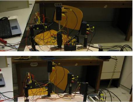
In the original set-up, the microphones were placed behind the space that was measured in. We will call this plane the y-z plane. We decided to surround the space that was measured in, because we noticed that the measurements in the x-direction were less stable than the measurements in the y- and z-direction. The difference between these set-ups is shown in figure 1, where you can see that mainly in the x-direction the microphones are more spread.

7

Laser & Galvano-mirrors

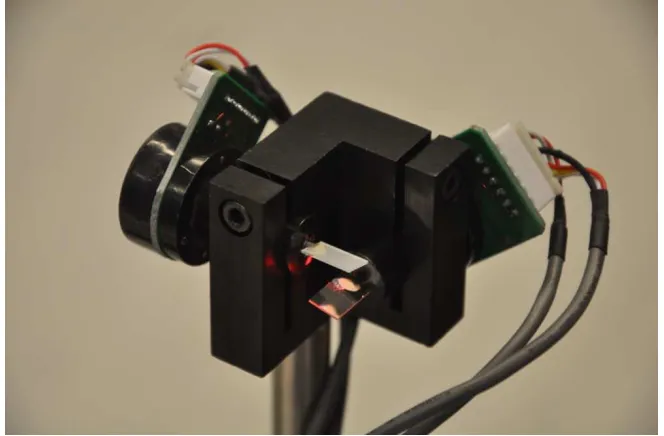
In our set-up we used a laser in combination with a two-axis galvano-mirror to target the mosquito after pinpointing its position using the acoustical localisation algorithm. The galvano-mirror is a device with two mirrors on two different axes which are mounted on two individually controllable motors. By rotating the mirrors the angle of incidence and therefore the angle of reflection of a beam aimed at the mirrors can be changed. Figure 2 shows the two galvano-mirrors.

Figure 2: The galvano-mirrors.

Because the mosquito is moving, a fast response of the mirrors is necessary. To characterise the dynamic response of the galvano-mirror the step response has been measured. We need the step response of the galvano-system, because we want to shoot as fast as possible at the location of the mosquito directly after measuring its location. After an initial targeting the galvano-mirrors will have to track the mosquito at a low speed. Therefore this behaviour can be considered quasistatic. To analyse how fast and precise this step response is, we measure the response of the motor that rotates the mirror. The step response can be characterized by multiple parameters, we will use the following:

- Step amplitude

- Settling time: the time it takes for the beam to coincide with the input value within the beam width

- Input delay: the time difference between the moment of input to the galvano-mirrors and the moment of motion of the galvano-mirrors

- Response time: the sum of the settling time and the delay - Overshoot: a non periodic ripple

The (step) response depends on the physical and electrical properties of the electronics, the motor and feedback sensors. We use a hardware that is a commercially available kit, AXJ-V20, used for laser shows. The available documentation is very limited, so we have to measure all of the above

8

The step response of the system can be attributed to the two parts of the system: the DAQ and the galvano-system. The galvano-system

controls the galvano-system. In order to separate the step response galvano-system the output of the DAQ will also be monitored. figure 3.

Figure 3: Galvano-system schematics

There are two possibilities for the input modes of the

has a linear angular response to the input or it has an angular response that is an inverse tangential The second response sounds counterintuitive from a physicist’s point of view, but since we use a system that is build to be used in laser

strange to have this response. For this application it is useful to

user only needs to enter the coordinates of the points of the image, without having to correc fact that the image is not projected on a spherical shell rather than on a flat screen.

however, the maximum angular deviation of the galvano difference between these two and just treat the system

The control between an input of spatial coordinates and the output of two voltages has

1 Coordinate transformation 2 Projection on calibrated plane 3 Transformation to voltage

Suppose that the mosquito is at (x,y,z).

(x’,y’,z’), this coordinate system has its centre on the galvano equilibrium position of the laser beam. Then we

projection is schematically shown in figure

have to transform these coordinates to an input voltage, V.

The step response of the system can be attributed to the two parts of the system: the DAQ and the system consists of an electronic circuit with feedback loop, which In order to separate the step response behaviour of the DAQ and the system the output of the DAQ will also be monitored. This set-up is schematically

There are two possibilities for the input modes of the galvano-system. The angle of the

response to the input or it has an angular response that is an inverse tangential second response sounds counterintuitive from a physicist’s point of view, but since we use a system that is build to be used in laser shows where you project an image on a flat screen, it strange to have this response. For this application it is useful to have a y-z input because then the

the coordinates of the points of the image, without having to correc fact that the image is not projected on a spherical shell rather than on a flat screen.

however, the maximum angular deviation of the galvano-mirror is small enough to neglect the difference between these two and just treat the system as a system with y-z input.

The control between an input of spatial coordinates and the output of two voltages has

Coordinate transformation Projection on calibrated plane Transformation to voltage

Suppose that the mosquito is at (x,y,z). The coordinates are transformed to a new coordinate system, his coordinate system has its centre on the galvano-mirror with the x’-axis parallel to the equilibrium position of the laser beam. Then we project the (x’,y’,z’) on a new plane, x’’.

shown in figure 4. If we know the coordinates in our calibrated plane, we coordinates to an input voltage, V.

The step response of the system can be attributed to the two parts of the system: the DAQ and the circuit with feedback loop, which

of the DAQ and the schematically shown in

system. The angle of the mirror either response to the input or it has an angular response that is an inverse tangential. second response sounds counterintuitive from a physicist’s point of view, but since we use a

shows where you project an image on a flat screen, it is not input because then the the coordinates of the points of the image, without having to correct for the fact that the image is not projected on a spherical shell rather than on a flat screen. In our case

mirror is small enough to neglect the input.

The control between an input of spatial coordinates and the output of two voltages has three steps:

a new coordinate system, axis parallel to the project the (x’,y’,z’) on a new plane, x’’. This

Figure 4: Scheme of the transformation to the coordinates on

Because the galvano-mirrors do not have a specified response they have to be calibrated first. In order to do this measurement the y’’(V) and

By finding the inverse of this relat to voltage transformation.

Complete device

The complete device consists of the two main parts: the galvano The coupling between these two sounds easy

transformed and becomes the input for the galvano The only problem that might occur during this

processing time is too high to hit the sound source. If this is the case we will try to reduce the processing time of both systems to make a functional bug zapper.

Figure 5: Scheme of the complete device

Error analysis

The errors in our system will be introduced by the two main parts of the set localisation will not be perfect, as we know from the original set

This will introduce the first error in our system, which will infl

The laser beam might also deviate from the position it is meant to be

galvano-systems. The errors in these two systems together have to be smaller than the mosquito, which results in a maximum error of 0.5 cm.

Scheme of the transformation to the coordinates on the calibrated plane

mirrors do not have a specified response they have to be calibrated first. In order to do this measurement the y’’(V) and z’’(V) responses are measured with a fixed x’’ distance By finding the inverse of this relation we get a proper V(y’’) relation to use in step 3 of our coordinate

The complete device consists of the two main parts: the galvano-mirrors and the sound localisation. The coupling between these two sounds easy, the output from the sound localisation

the input for the galvano-mirrors. This is schematically shown in figure 5. The only problem that might occur during this process is that the sum of the measuring and the

time is too high to hit the sound source. If this is the case we will try to reduce the processing time of both systems to make a functional bug zapper.

: Scheme of the complete device

errors in our system will be introduced by the two main parts of the set-up. The sound localisation will not be perfect, as we know from the original set-up for the sound localisation [1]. This will introduce the first error in our system, which will inflect the positioning of the laser beam. The laser beam might also deviate from the position it is meant to be as a result from an error in the

. The errors in these two systems together have to be smaller than results in a maximum error of 0.5 cm.

9 mirrors do not have a specified response they have to be calibrated first. In

(V) responses are measured with a fixed x’’ distance. ion we get a proper V(y’’) relation to use in step 3 of our coordinate

mirrors and the sound localisation. , the output from the sound localisation has to be

This is schematically shown in figure 5. measuring and the time is too high to hit the sound source. If this is the case we will try to reduce the

up. The sound up for the sound localisation [1]. ect the positioning of the laser beam.

10

Experimental aspects

Some parts of the set-up already existed. We used the same microphones as Ruud van Laar and Martijn van der Ouderaa. Since they were able to measure the location pretty well, we did not expect any problems on this point. The other thing we will use is the VI-file with the algorithm to calculate

the location.

Sound source

The easiest way to check if our smaller sound source works better than the sound source with a diameter of 5 cm is to test them both at multiple locations, especially near the microphones, and check whether the result is stable and whether it is reproducible. We also check if the smaller speaker is a good sound source for all of the frequencies of the sample we use.

Microphones & calibration

We optimize the positioning of the microphones by trial and error. We compare the signals of four different microphones with the same reference microphone, which gives us the chance to analyze the differences between the various positions we can choose. We calculate the DDOA between the microphones and compare that to the measured DDOA. We already know that there is a systematic mistake in this measurement [1], which we will obtain from these measurements.

The optimal set-up will be chosen by calculating the standard deviation and the average of the error in the DDOA. The error in the DDOA will be measured for multiple locations of the sound source for the four microphones compared to the reference microphone. The average of the error will be used as a constant correction of the DDOA, Ruud van Laar and Martijn van der Ouderaa already showed that there was an inexplicable error in the DDOA. The set-up with the smallest standard deviation is the most accurate in calculating the DDOA and therefore the best in calculating the location. We will try different ways of positioning the microphones, after doing the calculations for the previous set-up. For example, if we conclude that microphones close to each other give better results than the microphones far away from each other, we will try a new set-up with the four microphones closer to the reference microphone.

Galvano-mirrors

To measure the step response of the galvano-mirror a reference timescale is needed. There are multiple methods to do this. One could for example create a square wave and use a chopper to modulate the laser output and use this to scan the output signal. However, by using the fact that the system uses a two-axis mirror it is possible to create a reference timescale with one galvano-axis and use that to scan the response of the other galvano-axis.

11

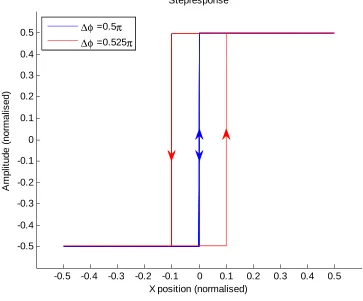
Figure 6: Simulation of a step response with and without phase difference.

The timescale on the x-axis follows from the frequency (f) of the triangular signal and the width (w) of the signal on the screen as shown in equation 1.

=

(1)

If the frequency is low enough to consider the square wave as a train of independent step functions, it is possible to say that the preceding step function does not influence the next step. We can check whether this is the case by looking if the line of the image is perfectly flat before it bends and use the described method to analyse the step response if the frequency is low enough. If there is some resonance present that is not fully damped before the next step and the resonance frequency is a multiple of the square wave frequency, this resonant signal can be amplified over multiple steps, thus making its influence seem bigger than it would be on not correlated random steps.

However, there might be some other disadvantages using this method. Equation 1 assumes that the galvano-mirror produces a perfect triangular output, this will not be the case. Because the derivative of a triangle is a square function the acceleration would have to be a delta peak at the top of the triangle, which is physically impossible. The triangular and the square wave are ½ π out of phase, which means that the angular velocity is constant at the point where the square wave changes sign. We assume that a constant angular velocity as input gives the galvano a constant angular response as output and that the settling time for the change in angular velocity is not too large. From these assumptions we can conclude that the deviation from a delta peak acceleration does not influence the timescale at x=0, but we will have to check if these assumptions are true.

If we align the input signal with a ∆φ=½ π, the actual projected image shows a slightly different

-0.5 -0.4 -0.3 -0.2 -0.1 0 0.1 0.2 0.3 0.4 0.5

-0.5 -0.4 -0.3 -0.2 -0.1 0 0.1 0.2 0.3 0.4 0.5 Stepresponse

X position (normalised)

A m p lit u d e ( n o rm a li s e d )

∆φ =0.5π

12

phase shift between the square wave and the triangle. This phase shift difference has been measured and documented as the input delay.

To measure the input delay in the triangular signal caused by the electronics we used a triangular signal as input signal. By using a photodiode coupled to an oscilloscope situated at the equilibrium position of the beam we measured the delay between the moment that the beam crossed the centre position and the moment that the electrical input to the galvano-system crossed the centre position. From this measurement we can conclude which part of the phase shift between the triangle function and the square function is attributable to the triangle function, if we assume that the lag of the detector is negligible.

Complete device

To test the functionality of the complete device, we will have to move the sound source through the measurable space with the speed of a mosquito. To test the device, we will capture a movie while moving the sound source through the measurable space. We will go through the measurable space repeatedly, and analyse whether the source is hit or not. We will also analyse 60 random shots to determine if the sample is hit or not. From these two analyses we can conclude how accurate our set-up is.

13

Results

Sound source

A disadvantage of the smaller speaker is the maximum volume of it. This gives us a lower SNR than we would have had when we would use the bigger speaker. On the other hand, its maximum volume is still higher than the maximum volume of one single mosquito, so it has be possible to detect a signal from the smaller speaker, otherwise the bug zapper would not work ‘in real life’.

When measuring far away (25-30 cm) from the microphones, there is no difference in the accuracy measurements between the two speakers. However, when it is moved closer to the microphones, the bigger speaker has a fluctuating, incorrect signal, while the smaller sound source still gives a reproducible measurement. Therefore we have chosen to use the smaller sound source with a diameter of 1.5 cm.

Microphones & calibration

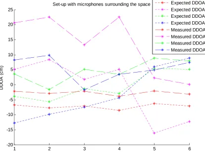
As mentioned in the theoretical aspects, our first guess is to place the microphones around the space that is measured in, because it could be possible that the result gets better by the spread in the microphones along the different axes. In figure 7 below, the measured DDOAs and the expected DDOAs are shown for six different positions. The measurements in this graph are shown without error bars, but these are very small. The measurements in the DDOA do not fluctuate more than ±0.05 cm.

Figure 7: Measured DDOAs compared to the expected DDOAs for the first set-up at six different locations.

1 2 3 4 5 6

-20 -15 -10 -5 0 5 10 15 20 25

Set-up with microphones surrounding the space

Measurements

D

D

O

A

(

c

m

)

14

The shape of the graphs is almost the same for the expected and the measured values, but there is a systematic error, which is much bigger than the one that Ruud van Laar and Martijn van der Ouderaa found in their set-up. [1]. While measuring the DDOAs, we had a small measurable space, so we decided to design a new set-up almost similar to the original set-up from Ruud van Laar and Martijn van der Ouderaa. [1]

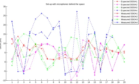
So in our next set-up, we placed the microphones behind the space we measured in. This gives the DDOAs as shown in figure 8 below. Here we see that the systematic error in the measurements is smaller, but we also see that there are more unexpected measurements, especially for microphone 3 and 4, these measurements do not seem to have a constant mistake in the DDOA. Since microphone 3 and 4 are further away from the reference microphone, we will try a third set-up, which is more similar to the set-up of the previous experiment. We place all of the microphones behind the measured space, but we bring them closer together, with a distance to the reference microphone of 15-20 cm.

Figure 8: The measured and expected DDOAs for the second set-up at twenty different positions

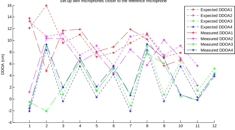
The third set-up gives us the results that are shown in figure 9. It can be seen that the systematic error decreases as the distance to the reference microphone decreases, but it is hard to say which set-up is the best.

1 2 3 4 5 6 7 8 9 10 11 12 13 14 15 16 17 18 19 20 -10

-5 0 5 10 15 20 25 30

Set-up with microphones behind the space

D

D

O

A

(

c

m

)

15

Figure 9: The measured and expected DDOAs for the third set-up at twelve different positions

Beside the measurements of the DDOA, there is another difference between these three different set-ups. The first set-up cannot measure the same points as the second and third set-up, because the two microphones that are placed in the space we would like to measure are not infinitely small. The microphones are little boxes and therefore distort the wave front so the sound source cannot be considered as a point source when the sound source is behind the microphone.

We calculate the average of the difference between the expected and the measured DDOA to estimate the systematic error and the standard deviation to choose between the second and third set-up, the results of this calculation are shown in the table in figure 10. The second set-up has a smaller measurable space, but might be more accurate compared to the third set-up.

Second set-up Third set-up

Average (cm) Stand. Deviation (cm) Average (cm) Stand. Deviation (cm)

DDOA1 -0.6 3.5 -0.6 3.9

DDOA2 -0.6 4.6 -2.5 3.4

DDOA3 -2.7 6.2 -1.0 4.1

DDOA4 -3.6 9.1 1.2 2.8

Figure 10: Table with average systematic errors and standard deviations.

The standard deviation is in both cases too big to get an accurate and precise result, so we will neglect a few of our measurements. This might sound a bit unusual, but it is possible that these locations were just out of our measurable space. The measurements we removed are all on the edge

1 2 3 4 5 6 7 8 9 10 11 12

-4 -2 0 2 4 6 8 10 12 14 16

Set-up with microphones closer to the reference microphone

D

D

O

A

(

c

m

)

16

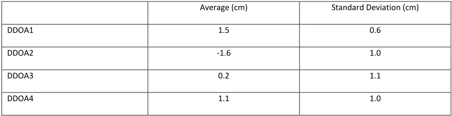
of the space we measured in. In figure 11 and 12 the graph with only the measurable locationsii and the table with the averages and standard deviation are shown. We will not use the second set-up, since the standard deviation in the second set-up is bigger than the standard deviation in the third set-up.

Figure 11: Measured and expected DDOA for the third set-up – only the measurable locations.

Average (cm) Standard Deviation (cm)

DDOA1 1.5 0.6

DDOA2 -1.6 1.0

DDOA3 0.2 1.1

DDOA4 1.1 1.0

Figure 12: Systematic errors that will be used to correct the localisation measurements in the third set-up

These results are good enough to use, but we still have more fluctuations than we had in the first set-up, where the microphones surrounded the space. Therefore we have designed a fourth set-up with the microphones surrounding the space we would like to measure in, a little bit different from the first set-up. We choose to make the space between the microphones bigger, in order to have the same measurable space as with the second and third set-up. This gave the results from figure 13 and 14.

ii

It is possible that at one location only one microphone is not measurable. The measurement of the DDOA is only dependent of the positioning of the reference microphone and the ‘measured’ microphone. Therefore we will end up with different numbers of measurements for the different microphones.

1 2 3 4 5 6 7 8 9 10

-4 -2 0 2 4 6 8 10 12 14

Set-up with microphones closer to the reference microphone - only measurable locations

Measurements

D

D

O

A

(

c

m

)

Expected DDOA1 Expected DDOA2 Expected DDOA3 Expected DDOA4

17

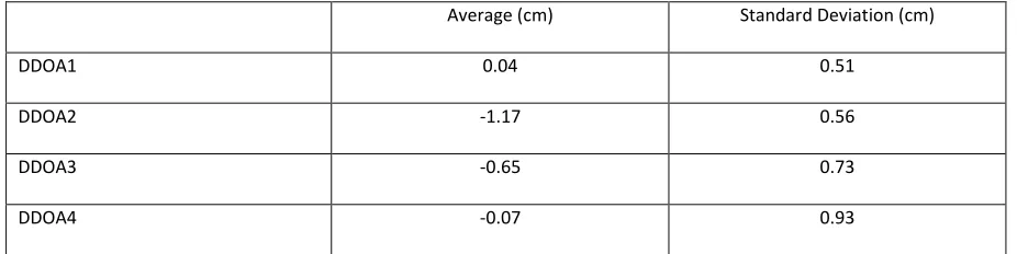
Figure 13: Measured and expected DDOA for the fourth set-up - only the measurable locations.

Average (cm) Standard Deviation (cm)

DDOA1 0.04 0.51

DDOA2 -1.17 0.56

DDOA3 -0.65 0.73

DDOA4 -0.07 0.93

Figure 14: Systematic errors that will be used to correct the localisation measurements in the fourth set-up

After analyzing the second, third and fourth set-up, it is still hard to choose between those two. Working through the error analysis of the algorithm we used [3], shows us that the relative mistake in the DDOA is important for the accuracy of the calculation of the location. Therefore, we will use the third and fourth set-up and choose the best, since the mistake in the DDOA is relatively small compared to the DDOA for both set-ups.

1 2 3 4 5 6 7 8 9 10 11 12 13 14

-15 -10 -5 0 5 10 15 20

Set-up with microphones surrounding the space - only measurable points

D

D

O

A

(

c

m

)

18

Sound localisation

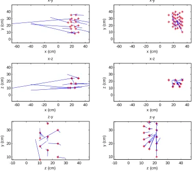
To determine how well the described set-ups work, we located the sound source at 18 different positions and measured the x-, y- and z-position of the source and compared this to the results of the sound localisation. The results for the third set-up are shown in figure 15 on the left. The results for the fourth set-up are shown in the graph below on the right.

Figure 15: Comparison of the real and measured position of the sound source, on the left the third set-up and on the right the fourth set-up. Real position marked using a red star, the blue line indicates where the point was measured.

It can be seen that the measurements with the surrounding microphones are more precise than the measurements with the microphones at y-z plane, especially in the x-direction. We can also see that the fourth set-up has a smaller measurable range, because the mistake in the localisation at the edge of the space is much bigger than the error at other measured points, as we already expected. If we neglect the points at the edge of our measured space we get the results from figure 16.

The fourth set-up has some advantages compared to the second and third set-up. The microphones are further away from each other, so the relative error is smaller and since they are more spread in the three directions, the errors are smaller for each of the directions.

-60 -40 -20 0 20 40

0 10 20 30 40 x-y x (cm) y ( c m )

-60 -40 -20 0 20 40

0 10 20 30 40 x-z x (cm) z ( c m )

-10 0 10 20 30 40

10 20 30 z-y z (cm) y ( c m )

-60 -40 -20 0 20 40

0 10 20 30 40 x-y x (cm) y ( c m )

-60 -40 -20 0 20 40

0 10 20 30 40 x-z x (cm) z ( c m )

-10 0 10 20 30 40

19

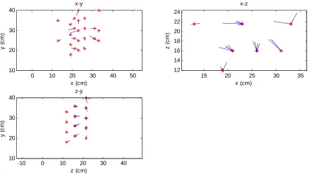
Figure 16: Comparison of the real and measured position of the sound source, with only the measurable points from the fourth set-up. Real position marked using a red star, the blue line indicates where the point was measured.

In the figure above the localisation of the measurable locations is shown. The average error in the x-direction is 1.1 cm (maximum 3.5 cm), in the y-x-direction it is 0.6 cm (maximum 2.6 cm) and in the z-direction it is 1.0 cm (maximum 2.4 cm). The measurable space is approximately spherical, with a diameter of 15-20 cm.

At first sight this might sound unsatisfying, because we did not improve the localisation as much as we hoped. On the other hand, our measurements are not averaged over multiple measurements, so we did reduce the processing time.

It seems like we will not hit every mosquito that comes into our bug zapper, but actually every mosquito will be measured more than once when it flies through our measurable space. We will further analyse the chance of surviving after the analysis of the galvano-mirrors when we combined the two systems.

0 10 20 30 40 50

10 20 30 40

x-y

x (cm)

y

(

c

m

)

15 20 25 30 35

12 14 16 18 20 22 24

x-z

x (cm)

z

(

c

m

)

-10 0 10 20 30 40

10 20 30 40

z-y

z (cm)

y

(

c

m

20

Galvano-mirrors

Various characteristics of the signal have been measured for twelve different frequencies (25Hz up to 300Hz in steps of 25Hz) and five different step amplitudes. The step amplitude is given in the angle between the start and end position of the mirror. As said before, the delay of the galvano-mirror is the phase difference between the triangular function and the square wave, the settling time is the time it takes to coincide with the input value. A typical response can be seen in figure 17. These characteristics are measured at the top and the bottom of the step function, in figure 17 a

measurement at the top of the step function is shown.

From these responses the average settling time and the average delay of the galvano-system are calculated, the settling time as a function of the amplitude is shown in figure 18, the delay in the galvano-mirror as a function of the amplitude is shown in figure 19 and the total response time as a function of the amplitude is shown in figure 20.

0 50 100 150 200 250 300 350

-0.1 0 0.1 0.2 0.3 0.4 0.5 0.6 0.7

Frequency (Hz)

T

im

e

(

m

s

)

Step amplitude 0.3416 rad (x-axis),top

Delay of galvano-system Settling time

21

Figure 18: Settling time as function of the step amplitude

Figure 19: Galvano-delay as function of the step amplitude

50 100 150 200 250 300 350 400

0.2 0.25 0.3 0.35 0.4 0.45 0.5 0.55 0.6 0.65

Step amplitude (mrad)

T

im

e

(

m

s

)

Settling time

Vertical axis (z) (top) Vertical axis (z) (bottom) Horizontal axis (x) (top) Horizontal axis (x) (bottom)

50 100 150 200 250 300 350 400

0.12 0.14 0.16 0.18 0.2 0.22 0.24

Step amplitude (mrad)

T

im

e

(

m

s

)

22

Figure 20: Total response time as function of the step amplitude

The first thing that we see from the three figures above is that the response time depends on the direction of the step. This simply shows that the feedback of the galvano is not symmetric, this can also be seen directly on the screen: at the bottom there is a slight overshoot increasing in size at higher frequencies. The second thing that we conclude from these graphs is that the two physical systems are not the same, because there is a difference in the response time between the two axes.

The delay of the triangular signal has been measured as well. In order to have an accurate timing the optical path was increased to about 3 m giving an image width or height of about 1 meter. This has been done because the beam is at shorter optical path lengths longer on the photodiode, making it harder to accurately measure the delay because the time on the photodiode can be of the same order as the delay. The delay has been measured at 100Hz and is shown in figure 21. There is a small error in this delay because of the time the laser is on the photodiode, this was about 25 μs.

The settling time of the DAQ has been measured to be about 15 μs, making it for practical purposes small enough to be neglected.

Axis Delay

X-axis 290±7 μs

Z-axis 280±5 μs

Figure 21: Delay of the triangular signal

All these measurements combined show that there is an input delay in the square wave of about 0.1 ms. The settling time, excluding this input delay is about 0.6 ms.

50 100 150 200 250 300 350 400

0.35 0.4 0.45 0.5 0.55 0.6 0.65 0.7 0.75 0.8 0.85

Step amplitude (mrad)

T

im

e

(

m

s

)

Total response time

23 The static behaviour of the galvano-mirrors has been measured as well. The results of these

measurements are shown in figure 22. The maximal deviation from the linear fit is about 0.7 mm, which is about half of the beam size, so we can assume that the galvano-system has a linear response over this voltage range.

Figure 22: Deflection as function from the input voltage at 42,8 cm away from the galvano-mirrors.

Complete device

We have analysed 60 shots of the twenty random paths. We can conclude that 8% of the

measurements will actually hit a mosquito, 44% is really close and might hit it if the mosquito flies in the right direction and 48% does not hit the mosquito.

In the 26 random ‘walks’ through our measurable space, the sound source is shot during 22 paths, which gives us a success rate of 85%. A random ‘walk’ is a path through the measurable space of approximately 20 cm.

-5 -4 -3 -2 -1 0 1 2 3 4 5

-8 -6 -4 -2 0 2 4 6 8

Voltage (V)

D

e

fl

e

c

ti

o

n

f

ro

m

c

e

n

tr

e

(

c

m

)

Beam deflection at 42,8 cm as a function of voltage

24

Discussion

Sound source & sample

The sound sample we used during our measurements was a short sample from a mosquito with malaria. Different species of mosquitoes flap their wings at other frequencies, but they might also have other frequencies when they make a turn or change their speed. To check whether this is the case, one could try to use the designed system with real mosquitoes. This also would solve the next question: is the sound of the mosquito loud enough to be detected by the five microphones? The Signal to Noise Ratio we had was relatively high, because we worked in a quiet place and did not talk during our measurements, so the system might be not functional in a crowded place.

Sound localisation

The sound source localisation method we used, was chosen because of the good results Ruud van Laar and Martijn van der Ouderaa had with these results. They tried one other algorithm, which was too slow. Though the algorithm is known as a fast method to calculate the location, there might be a faster algorithm.

Another disadvantage of this algorithm is the fact that it can only detect one mosquito at a time. Even worse, it cannot measure the location of one of the mosquitoes in the measurable space if there are more than one, because the correlation will be inflected by the different sound sources.

Galvano-mirrors

There were a few disadvantages of the galvano-system we used. The first problem was that the space you could aim the laser in depends on the angle of the mirrors, but the maximum amplitude we had was not big enough. However, if we would have had bigger amplitudes, the mirror would not be big enough to reflect the beam at high angles. To increase this space, we tried to put the galvano-system further away from the measurable space, but this would not be very useful in real life, since one would like to have the device as small as possible.

However, the response time and the precision of the galvano-system was very good, so maybe one could try to design a system with multiple galvano-systems to increase the space that can be hit or use optical demagnification.

Processing time

25

Laser

Since we only did a proof of concept in the first place, we did not look at the laser we would need to actually kill a mosquito. The amount of energy you need to kill a mosquito is 100 mJ according to E. Johanson[5], from which we can conclude that we would need a 100W laser, which is not eye safe. However, we have only found one article about the energy you would need to kill mosquitoes, which might not be trustworthy and they do not give enough details about the exposure time. To make a functional bug zapper more research to this laser would be needed. It is important to know how much power as a function of the exposure time is needed to kill a mosquito.

Complete device

26

Conclusion

We determined that with the described set-up it is possible to point a laser on the location of a sound source as long as its speed is not too high, though the accuracy is not very high.

Inaccurate measurements are mostly due to the sound localisation and not to the positioning of the laser. The measurements for the sound localisation can be done with 1 cm accuracy, which is too high to hit the mosquito every measurement. Eight percent of the measurements are precise enough to hit the mosquito.

27

Recommendations

During our project, we improved the bug zapper and proved that it is possible to pinpoint a source with a laser beam after determining the location. However, there are still some aspects of the bug zapper that could be improved.

- The measurable space is only a sphere with a diameter of 15-20 cm, more mosquitoes will be killed if this space is bigger.

- If there are two mosquitoes in (or close to) the measured the space, the system is unable to locate and shoot them, because the two signals will interfere. There might be a good solution to distinguish the two signals and locate them separately, but our set-up does not have this yet. To distinguish the two signals you might need more microphones and another algorithm than we used in our set-up, but the biggest problem will be the processing time of this new algorithm.

- In order to hit faster moving bugs, the processing time should be reduced even more, but this will have consequences for the accuracy of the measurements, as mentioned in the discussion.

There are also a few aspects that have to be considered before one should use this device in real life situations:

- If a mosquito is located, the laser will point at its location and will try to shoot the mosquito. If there is something on the path of the laser beam between the galvano-mirrors and the mosquito, this will be hit first. The laser you’ll need to kill mosquitoes will cause burns to other animals and humans as well. The system is therefore currently not suitable to use in your home. Maybe it is possible to use a sort of box around the system to protect the environment against the laser.

28

List of abbreviations

TDOA Time Difference Of Arrival

DDOA Distance Difference Of Arrival

29

References

[1] M. van der Ouderaa and R. van Laar, “The Bug Zapper”, Bachelor’s report University of Twente, 2013

[2] Alex Reisner, “Speed of Animals”, http://www.speedofanimals.com/animals/mosquito

[3] M. D. Gillette and H. F. Silverman, “A Linear Closed-Form Algorithm for Source Localisation From Time Difference of Arrival”, IEEE signal processing letters, vol. 15, pp. 1-4, 2008.

[4] R. H. Campbell, Composer, “Analysis of Mosquito Wing Beat Sound”. [Sound Recording]. Worcester Polytechnic Institute. 1996.