To a new hardware design methodology: A case study of the cochlea model

TO A NEW HARDWARE

DESIGN METHODOLOGY:

A CASE STUDY OF THE

COCHLEA MODEL

Floris van Nee

FACULTY EEMCS INCAS3

JAN KUPER JAN STEGENGA ANDRE KOKKELER RINSE WESTER

Contents

Abstract 2

Contents 3

1 Introduction 5

2 CλaSH and functional hardware design 7

2.1 Flaws in current design methodology . . . 7

2.2 Functional hardware design . . . 8

2.3 CλaSH . . . 9

2.3.1 The functions map, zipWith and fold . . . 9

2.3.2 The filter . . . 10

3 The cochlea 12 3.1 The real cochlea . . . 12

3.1.1 Structure . . . 12

3.2 The cochlea model . . . 14

3.2.1 Mathematical approach to the model . . . 15

3.2.2 Discretized recurrence relations . . . 22

4 Solving a tridiagonal system 26 4.1 Matrix inverse . . . 26

4.2 TDMA and Gaussian elimination . . . 28

4.2.1 Gaussian elimination for arbitrary matrices . . . 28

4.2.2 TDMA . . . 28

4.3 Cyclic reduction . . . 31

4.3.1 Cyclic reduction with back substitution . . . 31

4.3.2 Cyclic reduction without back substitution . . . 33

4.3.3 Optimizations . . . 34

4.4 Conclusion . . . 37

5 Transformations 38 5.1 Recurrence relations . . . 38

5.2 Lifting . . . 39

5.3 Folding . . . 40

5.3.1 Folding over time . . . 40

5.3.2 Folding equations . . . 41

5.3.3 Folding over n . . . 43

5.3.4 Hybrid cyclic reduction . . . 44

6 Implementation 46 6.1 Implementation requirements . . . 46

6.3 Conversion to CλaSH . . . 50

6.3.1 Generalization for M andN . . . 51

6.3.2 The CλaSH code . . . 51

7 Results 54 7.1 Simulation in Haskell . . . 54

7.1.1 40 dB sine input . . . 54

7.1.2 60 dB sine input . . . 55

7.1.3 80 dB sine input . . . 55

7.2 VHDL simulation . . . 55

7.3 Synthesis . . . 56

7.3.1 Xilinx ZYNQ-7000 board . . . 57

7.3.2 Xilinx 6VLX240TFF784 . . . 58

8 Discussion 60 8.1 Fixed-point . . . 60

8.2 Area usage . . . 60

8.3 ZYNQ-7000 . . . 61

8.4 6VLX240TFF784 . . . 62

8.5 Mathematical design methodology . . . 62

9 Conclusion 63

1 Introduction

Hardware design has always been a complex task considering the tradeoffs that have to be made between speed, area and development time. Because the size of transistors has been decreasing for a long time, thereby making larger designs possible, it is becoming an even more complex task to design hardware correctly. Furthermore, the advent of FPGAs have made hardware design more widespread, because they provide a low-cost solution for many problems where a high-performance design is required. Therefore, it is vital to have a design process with support for these tradeoff factors efficiency and development time.

In the field of hardware design the design problem often consists of a specification which is written in a mathematical form. In order to end up with a synthesizable design the following methodology is often used: generally, a model of this specification is created in, for example, Matlab for validation, after which an implementation in a low-level language like C is created. As a last step, the C code is made suitable for implementation on hardware, for example by using it to write VHDL. This last step is usually done manually, but a lot of research currently focuses on automating this C to hardware conversion [1]. Also, SystemC is often used to translate the C code to as it provides slightly higher abstraction levels [2].

In order to see the possible advantages of a new design methodology, it is important to notice the flaws of the current design methodology. Most importantly, in the translation between the mathematical form and Matlab/C, a lot of important information is lost. Data dependencies, essential information for parallelisation, are clearly present in a mathematical form, but cannot be easily extracted from Matlab/C code [3]. Tools which automatically try to transform C code to VHDL are often restricted to a small subset of C for which it is possible for the tools to infer the data dependencies [1]. In other cases, the tool will generate either inefficient VHDL or it will not be able to process it at all. When engineers work on manually translating the C implementation in VHDL, they often have to infer these data dependencies from Matlab/C code themselves. This is a cumbersome and error-prone task which can easily lead to the introduction of bugs.

The specific case study that is presented is about the implementation of a model of the cochlea. The cochlea is the auditory portion of the inner ear and a lot of research has previously been done on obtaining accurate mathematical models of the cochlea. Several models exist, some more complex than others, and in this case study we have chosen to focus on the one-dimensional cochlea model with linear damping distribution [5]. INCAS3 is doing research on the cochlea model itself as well as on the implementation on several different platforms and on the use of the model for sound recognition. Investigating the implementation of the model on an FPGA was a natural next step as the model has a large potential for parallel execution and this is one of the areas in which FPGAs are strong. On top of that, because all processing is done locally on the FPGA instead of processed in a data centre, there are less privacy issues as not all data needs to be transmitted to a central server. Last, FPGAs are generally more energy efficient than software and they provide a first step to an ASIC design which are even more energy efficient. INCAS3 generally does hardware design using the traditional approach with Matlab, C and VHDL, but is interested in the new approach as they have also observed problems with the traditional approach.

Therefore, the purpose of this research is two-fold. First, a new design methodology using CλaSH is tested with a case study to determine its strong and weak points. Second, by doing this case study valuable information about the implementation of the cochlea model on an FPGA is obtained. This allows us to formulate the reserach questions as follows:

• How well is the new design methodology and CλaSH suited for a large design project like the cochlea model?

• Is the FPGA a suitable platform for implementation of the linear cochlea model in terms of performance?

Factors that play a role in the first research question include the difficulties that arise when doing the mathematical transformations, how well the speed/area tradeoff can be considered in the early design stages with the mathematical formulas and if the current state of the CλaSH implementation is stable enough for a case study this size. For the second research question, the main factors are whether or not there is enough parallelism to exploit and whether the algorithm is not too complex to fit on an FPGA. As this is largely dependent on conditions like the type of FPGA and settings of the algorithm, we have formulated several specific implementation conditions which can be found in chapter 6.

2 C

λ

aSH and functional hardware design

This chapter provides an introduction to the functional hardware design methodology using CλaSH. The first two sections focus on the design methodology and the theoretical advantages while the third section introduces CλaSH as a hardware description language.

2.1 Flaws in current design methodology

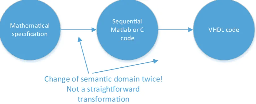
Traditionally, the hardware design methodology, especially in the signal processing domain, consists of several steps from specification to VHDL. Several improvements and abstraction layers have been suggested over the years, but the concept remains the same [2]. A graphical representation of this design methodology can be found in figure 2.1. The process always starts with a specification that needs to be implemented on hardware. The specification is often written down in a purely mathematical way. As a first step, this mathematical specification is converted to sequential code in a language like C. The main problem with this conversion is that the semantics of a C-like language do not match the semantics of the original mathematical specification. Because of this, a translation between the two is not straightforward. The largest difference between the two is called referential transparancy versus referential opaqueness [6]. In mathematics, expressions with the same parameters always yield the same result. Therefore, it is possible to replace an expression with its value. It is said to be referentially transparent. This is not the case in C, as expressions can have side-effects and they can yield different results each time they are evaluated. It is said to be referentially opaque. To validate correctness of the translation between mathematics and C, extensive verification is required. After the design has been verified, the second step is to translate the C-like language to RTL-style VHDL or Verilog code. Again, the semantics of VHDL and C-like code do not match, which leads to more time-consuming verification and the possible introduction of unwanted design faults.

Mathemacal specificaon

Sequenal Matlab or C

code

VHDL code

Change of semanc domain twice!

Not a straigh"orward

transformaon

Thus, the main flaw in the current design methodology is the need to change semantic domain twice: first from mathematics to sequential C-like code, then from C-like code to RTL-style VHDL or Verilog. Because the translation between these domains is not straightforward, extensive verification has to be performed. Also, the intermediate sequential C-like code is not strictly needed in the design process. This intermediate step mostly exists due to the fact that generally some implementation of the algorithm in software is required for verification, and that the most-used languages for software are sequential C-like languages. This generally makes it the first choice for implementation in software. However, these kind of languages are not suited for translation to hardware, because, as mentioned in the previous paragraph, there is a semantic mismatch between C-like languages and VHDL.

Therefore, we would like to have a methodology which includes the possibility to verify a software version of the algorithm, but not with a sequential C-like language. We would like to avoid the semantic mismatch, as discussed in the previous paragraphs, to reduce the effort required for verification and to reduce the possibility of introducing design faults.

2.2 Functional hardware design

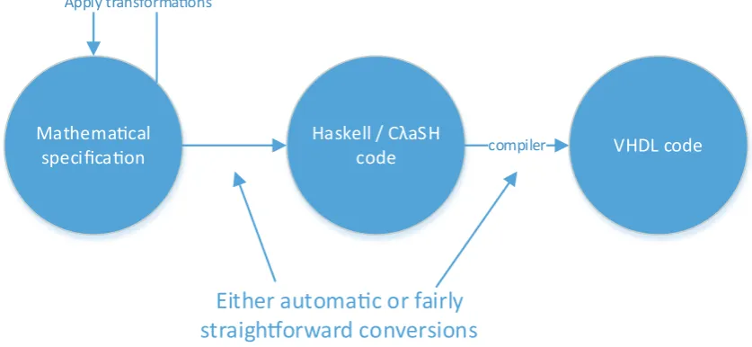
The design methodology that is tested in this thesis is based on the functional programming language Haskell and the CλaSH compiler [7] [4]. A graphical representation of this method-ology can be found in figure 2.2. It allows for software testing of the algorithm, but does not have the disadvantage of having to manually switch semantic domain twice. Instead, the mathematical specification can be rather straightforwardly converted to a Haskell program. The conversion between the mathematical specification and Haskell is less error-prone than the conversion between the specification and a C-like language, because the semantics of Haskell and mathematics largely match. Haskell has referential transparancy and functions in Haskell only specificy true data-dependencies, just like mathematical functions, which means that parallelism remains exposed. This is important, as in the transformation to hardware this parallelism needs to be exploited. In programs written in C, the designer needs to manually introduce parallelism again.

Mathemacal specificaon

Haskell / CλaSH

code compiler VHDL code

Apply transformaons

Either automac or fairly

straigh"orward conversions

Figure 2.2: The functional design methodology

A processor is sequential in nature and the GHC compiler (Glasgow Haskell Compiler), the most widely used compiler for Haskell, can be used to compile Haskell programs to code which runs on a processor. This step is thus done automatically instead of manually in the case of translating the mathematical model to C.

When the mathematical specification has been translated to Haskell, the next step is to find transformations on the specification for optimizations. These transformations can be written down mathematically, allowing us to prove the correctness of the transformations at any point in the design process. Transformations can be as simple as operand interchangement of associative functions, but more complex transformations can also be done some of which are used and described in chapter 5.

The resulting specification in Haskell can then be given to the CλaSH compiler, which takes a subset of Haskell as input and produces VHDL-code of that design as output. Once the VHDL-code is obtained, it can be used with standard synthesis tooling. The choice for VHDL as output is solely made, because of the large number of existing synthesis tools.

As can be seen in figure 2.2, the big advantage of this methodology is that every step in the process is either performed by the compiler, mathematically provable or fairly straightforward. This is a huge advantage over the old methodology in figure 2.1, where both steps need to be done manually and are not straightforward at all.

2.3 C

λ

aSH

CλaSH is the compiler which takes a Haskell program and translates it to VHDL. Not every Haskell program can be translated to VHDL though. Only a subset of Haskell is supported in the current CλaSH version. Restrictions include fixed-point calculations only, no recursion and vectors are used instead of lists. This section aims to introduce CλaSH with a small example of a FIR-filter as also described in [3].

2.3.1 The functions map, zipWith and fold

In the functional programming language Haskell there are three functions which are used very often. These three functions operate on lists and all of them also take a function as one of their arguments, which means they are higher order functions. The functions are: map, zipWith andfold.

The functionmaptakes a functionfas input and a list of elementsxsand applies the function fto every element in xs. The function f takes one input of type a and outputs a value of typeb(possibly aequals b). Thus, the type of map is:

1 map :: (a -> b) -> [a] -> [b]

x0 x1 · · · xn−1

f f · · · f

The functionzipWithis similar tomap, except that it takes a binary functionfas input and two lists,xsandys, instead of one. It then applies the function fpairwise to every element inxsand ys: it zips them together. The type of zipWithis:

zipWith :: (a -> b -> c) -> [a] -> [b] -> [c]

x0y0 x1y1 · · · xn−1yn−1

∗ ∗ · · · ∗

w0 w1 · · · wn−1

The function fold reduces a list of elements to a single value. In order to that, it takes a list of elementsxsto reduce, a starting valuezand a functionfwhich takes two inputs and produces one output. Reduction will start at on end of the list and at each step the result of the last element and the next element will be the input to the functionf. The type of fold is:

fold :: (a -> b -> a) -> a -> [b] -> a

w0 w1 · · · wn−1

+ + · · · +

0 z

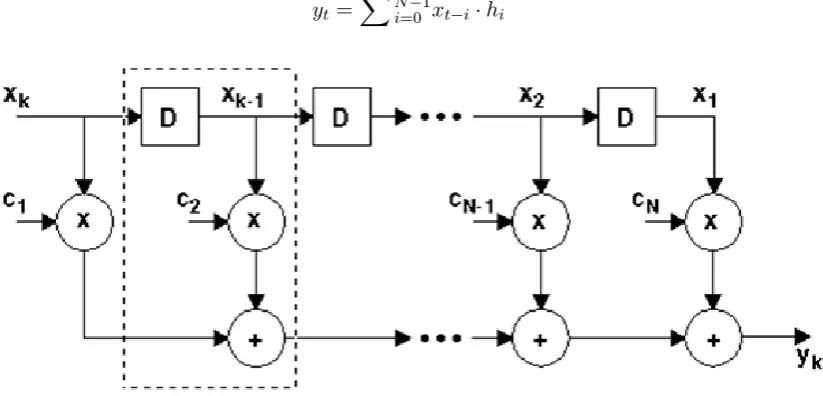
2.3.2 The filter

A FIR-filter is defined mathematically as follows:

yt=

∑_N−1

i=0 xt−i·hi

Figure 2.3: Structure of a FIR-filter

dotp xs hs = vfoldl (+) 0 (vzipWith (*) xs hs)

The FIR-filter can then be defined as:

fir coeffs xs = ys where

ys = dotp coeffs wxs wxs = window xs

3 The cochlea

3.1 The real cochlea

The word cochlea is the classical Latin word for inner ear. The human ear, or any mammalian ear for that matter, can be divided into three parts: the outer ear, the middle ear and the inner ear. A schematic of the complete human ear can be found in figure 3.1. Sound waves travel through air into the external auditory canal, which is part of the outer ear. The middle ear, with the malleus and incus acts as a conversion between the sound pressure in air in the outer ear and fluid displacement in the inner ear. The cochlea then converts this fluid displacement into signals that travel to the brain.

Figure 3.1: Schematic of the human ear [8]

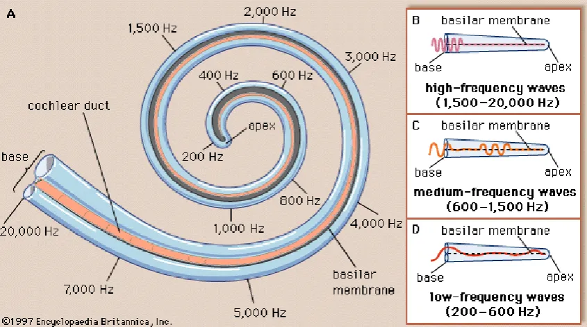
3.1.1 Structure

which the upper one is oval and the lower one round. The main parts of the cochlea include (see figure 3.2):

• The scala vestibuli, the scala which lies superior to the cochlear duct. This has the oval window at the base.

• The scala tympani, the scala which lies inferior to the cochlear duct. This has the round window at the base.

• The scala media, also called cochlear duct, which lies in between the scala vestibuli and scala tympani. It has a high potassium ion concentration.

• The helicotrema, the location where the scala vestibuli and scala tympani merge at the apex.

• The basilar membrane, the membrane that seperates the scala media from the scala tympani.

• The Reissner’s membrane, the membrane that seperates the scala media from the scala vestibuli.

• The Organ of Corti, the part taking care of the transduction mechanism. It is located on the basilar membrane. The mechanics of this are complex and not relevant for this thesis and will thus not be discussed further.

Figure 3.2: Structure of the cochlea [5]

For the model that is described in the next section, the important part of the cochlea is the basilar membrane together with the Organ of Corti. These two together are called the cochlear partition.

Figure 3.3: Structure and frequency response of the cochlea

3.2 The cochlea model

Several models of the cochlea exist [5] [9] [10]. In this section, a visual approach will be given for the models with linear and non-linear damping distribution as described by Duifhuis [9].

Both models are a drastical simplification of the real cochlea, because the real cochlea is a very complex organ. A drawing of the model can be found in figure 3.4. Simplifications of the real cochlea compared to the model include:

• The cochlea is rolled out. Instead of a spiral form, it is now stretched out in one dimension.

• The scala media and scala vestibuli are lumped together. The exact reason why this is possible is out of the scope of this thesis, but is based on the properties of the Reissner’s membrane and the hydromechanical properties of the different fluids.

• The cochlea ducts have rigid walls. Communication can only happen through its oval and round windows.

• The cross-sectional areas of the ducts are assumed to be constant over length and are approximated by rectangles.

• The fluid is assumed to be inviscid and linear.

• The cochlear partition is assumed to be split up in small sections. Every section can be modelled as a mass-spring-damper system with different parameters. Thus, every section has a different resonance frequency.

Figure 3.4: The simplified linear cochlea model [5]

One part that has been left unspecified yet is the input to the model. Sound waves first travel through the outer ear and middle ear before arriving at the cochlea. Therefore, even though the model only treats the cochlea, it is still important to have an idea of what happens to the sound waves before they reach the cochlea. The effect of the outer ear is assumed to be negligible and is thus ignored in the model. The middle ear has a simple mechanical transfer and is thus assumed to be linear in this model. Within INCAS3, there is currently research on the effects of the middle ear on the input, because it can be modelled more precisely than a linear transfer. However, for simplicity the model described here uses the linear transfer function.

3.2.1 Mathematical approach to the model

Figure 3.5: Example of damping distributions for both the non-linear model (a) and linear model (b) [10]

Examining this circuit leads to equations for the pressure at different points of the membrane. These equations are made dimensionless in order to bring all values within a small range to facilitate calculation in fixed point. Then, the equations for calculating the speed and distance of the membrane when the pressure is known are given. These are also made dimensionless. These equations still have a partial differential, thus they have to be discretized. The result of this discretization is a set of discretized recurrence relations for the speed and distance of the membrane.

Electrical equivalent

Van den Raadt describes the model as an RLC-circuit withN+1oscillators [5]. Every oscillator corresponds to one of the small sections of the cochlear partition. An oscillator has a current through it. The current defines the speed of the membrane at that point. The charge (integral of the current/speed) defines the relative distance of one point of the membrane to position zero. We are interested in these two values for every oscillator in the membrane. The positions

n= 0(input signal) andn=N (last oscillator) are handled somewhat differently, thus in this section we only focus on the oscillators between the first and last position, which means that

0< n < N. For the mathematical derivation forn= 0andn=N we refer to Van den Raadt [5].

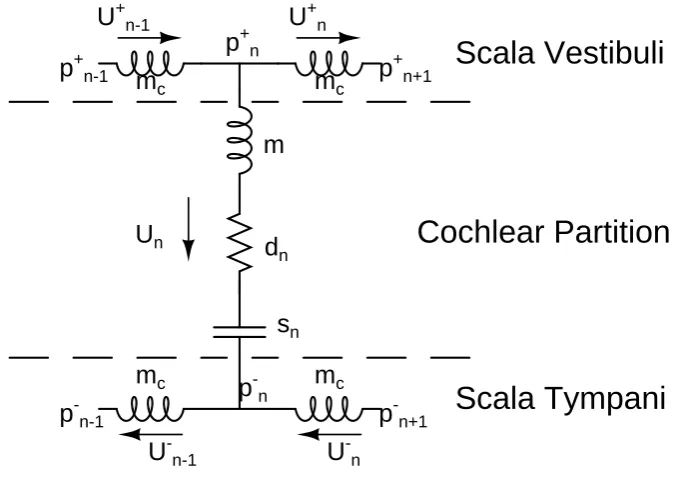
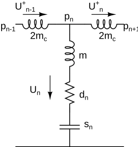
One such oscillator can be described by the network in figure 3.6. With some circuit equations this can be rewritten to the simplified version in figure 3.7. While the figure suggests an electrical network, the names in the figure correspond to values in the actual model. Note that even though we use electric-domain analogy, we retain the mechanical-domain variable names. The following are used in the figures:

Note that the only thing that couples two oscillators is the fluid movement. Writing Kirchhoff Voltage Law (KVL) and Ohms law equations for pointnin figure 3.7, using the definition of an inductor, gives us the voltage over two of the inductors:

pn−1−pn= 2mc

∂U_n+₋₁

∂t (3.1)

pn−pn+1 = 2mc

∂U_n+

Name Electrical equivalent Mechanical definition

Un current through pointn

downwards

speed of the membrane at

Yn charge at pointn position of the membrane at oscillatorn

U_n+₋₁,U_n+ electrical current fluid flowing to point n from the left and current flowing to pointn+ 1from the left respectively

pn−1,pn,pn+1 voltage at said points membrane pressure at said points

mc induction acoustic mass of the cochlea fluid between two

os-cillators

m induction acoustic mass of oscillatornof the membrane

dn resistance damping at oscillatorn

sn capacitance area of oscillatorn

Table 3.1: Variable names and their electrical-domain equivalents

m

m

m

m

d

s

m

U

U

U

U

U

p

p

p

p

p

p

Cochlear Partition

Scala Vestibuli

Scala Tympani

Figure 3.6: Oscillator for 0< n < N

Subtracting equation (3.2) from equation (3.1) and using Kirchoff Current Law, which states that the sum of the currents flowing from/to a node needs to be zero, leads to:

pn−1−2pn+pn+1 = 2mc

∂Un

∂t (3.3)

This can be simplified further by first writing the voltage at pointpnas the sum of the voltage

over the capacitor, resistor and inductor with inductancem:

pn=m

∂Un

∂t +dnUn+sn

∫

Undt (3.4)

Here we define the last part of this equation asGn, because it will make the final expression

2m

2m

m

d

s

U

U

U

p

p

p

Figure 3.7: Simplified oscillator for0< n < N

Gn=dnUn+sn

∫

Undt (3.5)

=dnUn+snYn (3.6)

AndGn is substituted in equation (3.4):

pn=m

∂Un

∂t +Gn (3.7)

Slightly rewriting this with basic algebra leads to an equation for ∂Un

∂t :

∂Un

∂t =

pn−Gn

m (3.8)

Equation (3.8) can be substituted into our previous equation (3.3):

pn−1−2pn+pn+1 = 2mc

pn−Gn

m (3.9)

p_n−1−2pn+pn+1 = 2 mc

mpn−2 mc

mGn (3.10)

pn−1−2(1 + mc

m)pn+pn+1 =−2 mc

mGn (3.11)

Equation (3.11) is the main equation that needs to be solved in order to calculatepn. There is

of the computation is already becoming clearer at this point. First, Gn can be calculated

using state variables Un and Yn for every 0 < n < N. Then, the right hand side can be

calculated completely by multiping with−2mc

m. Once this is known, we have to solve all these

equations as a system of linear equations. The result of this computation yields all valuespn.

As mentioned before, there is also an oscillator atn=N and an input signal atn= 0. These are handled a little bit differently, but the principle is the same. It results in one large system of equations for0≤n≤N for a total of n+ 1equations.

Dimensionless equations

These equations contain values with a large range. Some, like the time step for example have a value of 10−3, while others have much lower values. In order to perform the calculations more precise it is essential that the dynamic range of all values is as small as possible. This can be done by dividing the equations by some predefined constants with the same dimension. Afterwards, the equations are said to be dimensionless. Van den Raadt defines the following variables and chose a suitable value by using experimental data [5]. We use the tilde on top of a parameter to indicate that it is dimensionless. For example, ϕ˜n is the dimensionless

counterpart of ϕn. Parameters with a hat are used to indicate that these are used to make

equations dimensionless.

b

t0= 1·10−3s (3.12)

b

x0= 35·10−3m (3.13)

b

y0= 1·10−9m (3.14)

Thebt0 is used to make the quantity of time dimensionless. The bx0 is used to make the static quantities for the length of the basilar membrane dimensionless, like the ∆X which arises when discretizing the cochlea. To make the dynamic quantities dimensionless, like speed and pressure of the membrane,y0b is used. For the full derivation, we refer to Van den Raadt [5]. In this document we present their main findings with a short derivation.

First, we defineϕas:

ϕn=

pn

ms

(3.15)

ϕn has unit _sm2, because mc is a model parameter with unit m and pn is in Pascal (see Van

den Raadt for derivation), thus in order to make it dimensionless it needs to be multiplied with bt2₀ and divided by by0. Definingϕ˜as the dimensionless ϕ, we get:

ϕn= b

y0

b

t2 0

˜

ϕn (3.16)

Now we expand our previous definition ofGn (equation (3.6)):

Gn=dnUn+snYn (3.17)

In this formula, bBM is the width of the basilar membrane, ∆X the distance between two

oscillators andun (unit m_s) and yn (unit m) respectively the speed and distance per area of

the basilar membrane.

We can make equation (3.18) dimensionless by making the following terms in the equation dimensionless:

yn=y0by˜n (3.19)

∆X =x0b ∆ ˜X (3.20)

t=bt0˜t (3.21)

d dt = 1 b t0 d

d˜t (3.22)

And using equation (3.19) and equation (3.22),un can also be made dimensionless:

un=

dyn dt = b y0 b t0 d

d˜ty˜n (3.23)

= yb0

b

t0

˜

un

These can be substituted into equation (3.18) to obtain a new equation forGn:

Gn=bBM ·x0b ·y0b ·∆ ˜X(

dn

b

t0u˜n+sny˜n) (3.24)

Using this new definition ofGn (unit m

2

s2), we define the dimensionless gn:

gn=

bt2₀

b

y0 · Gn

ms

(3.25)

As a last step before introducing our final equation for the normalized pressure ϕ˜n, we note

that 2mc

m can be normalized to:

2mc

m =α

2

xn∆ ˜X

2 _(3.26)

We refer to Van den Raadt voor de full derivation for this step. The important part is that

αxn is a parameter which depends on several other parameters in the model, like membrane

width, density of the cochlear liquid and the area of one oscillator.

It is now possible to substitute equations (3.15), (3.16), (3.25) and (3.26) into equation (3.11) to obtain the dimensionless equation forϕ˜n for 0< n < N:

˜

ϕn−1−(2 +α2xn∆ ˜X

2_{) ˜ϕ}

n+ ˜ϕn+1 =−α2xn∆ ˜X

2_g

n (3.27)

Withgndefined as:

gn=

bBM ·bx0·∆ ˜X

ms ·

System of equations

Just like equation (3.11), equation (3.27) results in a system ofN+ 1 equations (with n= 0

and n = N slightly different than shown here, but similar in principle) that can be solved by any method of solving systems of equations. Van den Raadt proved that the system is diagonally dominant. Furthermore, because every equation in the system only depends on its neighbours, it is a tridiagonal matrix system which can be solved efficiently. The resulting matrix-vector equation can be written as:

A·ϕϕϕ˜=rrr (3.29)

Here, the right-hand sidern and the main diagonalan of A(for 0< n < N) are defined as:

rn=−α2xn∆ ˜X

2_g

n (3.30)

an=−(2 +α2xn∆ ˜X

2_{) (3.31)}

The matrixA is defined as:

A=             

−(1 +α0∆ ˜X01) 1 0 0 0

1 a1 1 0 0

. .. ... . ..

0 1 an 1 0

. .. ... . ..

0 0 1 aN−1 1

0 0 0 1 −(1 +α2_xN∆ ˜X2+ 4ˆx0∆ ˜X

πh+4ˆx0∆ ˜X              (3.32)

The two diagonals next to the main diagonal ofAare filled with 1, which shows the dependency on the neighbour oscillator, while the rest of the matrix is 0. Different methods to solve this system of equations are discussed in chapter 4.

Equations to integrate

The result of solving the system of equations will be the dimensionless pressure for every oscillator,ϕ˜n. Now, this result can be used to calculate the speedUn and distanceYn. Recall

equation (3.7):

pn=m

∂Un

∂t +Gn (3.33)

This equation can be rewritten to:

∂Un

∂t =

pn−Gn

m (3.34)

Also, asYn is defined as the integral ofUn, we have:

∂Yn

∂t =Un (3.36)

Equations (3.34) and (3.36) need to be made dimensionless again. Again, for full details of this step see the document by Van den Raadt.

Equation (3.34) can be made dimensionless by substituting equations (3.16), (3.22), (3.23) and (3.25) and simplifying the resulting expression. This results in:

∂u˜n

∂˜t = ˜ϕn−gn (3.37)

Equation (3.36) for Yn can be made dimensionless by substituting equations (3.19), (3.22)

and (3.23) and simplifying the resulting expression. This results in:

∂y˜n

∂t˜ = ˜un (3.38)

Thus, now we have the two dimensionless equations which need to be integrated over time. These equations are for oscillators at position 0 < n < N. The equations for n = 0 and

n=N are slightly different, but have a similar form. For these equations we refer to Van den Raadt.

3.2.2 Discretized recurrence relations

The current model is already discretized for space: the basilar membrane is divided into sections where every section is modelled by an RLC-circuit as described in the previous section. However, the model is not discretized for time yet. Equations (3.37) and (3.38) contain integrals over time which need to be discretized in order to compute them.

To discretize these equations, we first recall the definition of the partial differential operator:

∂f(t)

∂t = lim∆t→0

f(t+ ∆t)−f(t)

∆t (3.39)

A simple method of discretizing this partial differential operator is by taking a sufficiently small value for∆tto obtain an estimate of above equation without the limit. This method can be applied to equation (3.37) and (3.38) to eliminate the partial differential. As values like u˜n

andy˜n also depend on the time,˜t, we write u˜˜t,n andy˜˜t,n from now on to make it explicit:

∂u˜t,n

∂˜t = ˜ϕ˜t,n−g˜t,n =⇒

lim

∆˜t→0

˜

u˜_t+∆˜t,n−u˜˜_t,n

∂y˜t,n

∂˜t = ˜u˜t,n =⇒

lim

∆˜t→0

˜

y˜_t+∆˜t,n−y˜˜_t,n

∆˜t = ˜u˜t,n (3.41)

By choosing ∆˜t small enough, we can obtain the discretization of time. This leads to a sequence of time steps. To simplify notation further, we now use thetas an integer indicating the time step. Thus, timestep t and t+ 1, to consecutive timesteps, differ by ∆˜t in actual dimensionless time. This leads to:

˜

ut+1,n−u˜t,n

∆˜t = ˜ϕt,n−gt,n =⇒ (3.42)

˜

ut+1,n = ˜ut,n+ ∆˜t·( ˜ϕt,n−gt,n)

˜

yt+1,n−y˜t,n

∆˜t = ˜ut,n =⇒ (3.43)

˜

yt+1,n = ˜yt,n+ ∆˜t·u˜t,n

These two equations are the discretization of equation (3.37) and (3.38), which means that we now have a fully discretized model for the cochlea. For completeness, let us recap all recurrence relations now. Note that all recurrence relations are now indexed both for time,t, and space,n. The boundaries for tand nare specified for all recurrence relations. Wherever the equations forn= 0andn=N are equal to those for0< n < N, the boundaries reflect that. The boundary is set to0< n < N wherever the equations are not equal. In this case, we specify the relation forn= 0 andn=N, but do not give a formal derivation. We refer to Van den Raadt for the derivation of the equations forn= 0 andn=N.

Note that we have equations for gt,n, rt,n, ϕt, n˜ , ut,n and yt,n. The dependencies between

these different equations is visualized in figure 3.8.

calc gt

g

_t

r

_t

ϕ

_t

u

t-1

y

_t-1

u

t

y

_t

Figure 3.8: The data dependencies for different time steps between the equations

˜

u0,n = 0 0≤n≤N (3.44)

˜

y0,n = 0 0≤n≤N (3.45)

The values for the next step are then given by the following recurrence relations:

The relationship for gt,n

Recall equation (3.28):

gn=

bBM ·bx0·∆ ˜X

ms ·

(dntˆ0u˜n+sntˆ20y˜n) (3.46)

In order to simplify the equations, we define:

Un=

bBM ·bx0·∆ ˜X

ms ·

dnˆt0 0< n≤N (3.47)

Yn=

bBM ·bx0·∆ ˜X

ms ·

snˆt20 0< n≤N (3.48)

Both Un and Yn are only dependent onn and are constant over time, which is why they are

only indexed withn. The equation forn= 0is not shown, but is similar. Substituting this in (3.28) and adding the index over time forg, we get:

gt,n=Un·u˜t−1,n+Yn·y˜t−1,n t≥1∧0≤n≤N (3.49)

The relationship for rt,n

We definert,nto be the right-hand side of the system of equations that needs to be solved at

a given timestep. Recall equation (3.27):

˜

ϕn−1−(2 +α2xn∆ ˜X

2_{) ˜ϕ}

n+ ˜ϕn+1 =−α2xn∆ ˜X

2_g

n (3.50)

First, we define Rn for simplicity, just like Un and Yn were defined. See Van den Raadt for

the calculation ofRn forn= 0 andn=N. For now, we assume that these values exist.

Rn=−αx2n∆ ˜X

2 _{0< n < N (3.51)}

The first oscillatorn= 0 is handled differently than the other elements here, because it takes into account the current inputit. SubstitutingRn into (3.27):

rt,0 =R0·(it+gt,0) t≥1 (3.52)

Solving the equation

With the relation for the right-hand side given, it is now necessary to solve the system of linear equations. Several methods exist which are discussed and compared in chapter 4. For now, it is important to understand that the following equation needs to be solved forϕ˜t(see equation

(3.29)), whereAis a tridiagonal matrix,rrrt a vector for all values ofrt,n at a certain timestep

andϕϕϕ˜_ta vector for all values of ϕ˜t,n which need to be calculated.

A·ϕϕϕ˜t=rrrt t≥1 (3.54)

The relationship for ut,n

The discretized equations forut,nis already given in equation (3.43). Recall thatut,nrepresents

the speed of the membrane at pointn. One minor adjustement is made to the equation for

ut,n. Vn is defined (ms andmsm are parameters of the model):

V0 = ms

msm ·

∆˜t (3.55)

Vn= ∆˜t 0< n≤N (3.56)

This is substituted into equation (3.43). Note that the the case for n = 0 is different, as it also takes into account the input.

˜

ut,0 = ˜ut−1,0+V0·( ˜ϕt,0−gt,0−it) t≥1 (3.57)

˜

ut,n= ˜ut−1,n+Vn·( ˜ϕt,n−gt,n) t≥1∧0< n≤N (3.58)

The relationship for yt,n

The equation foryt,n, the displacement of the membrane at pointn, remains equal to equation

(3.44):

˜

yt,n= ˜yt−1,n+ ∆˜t·u˜t,n t≥1 (3.59)

The complete set of equations has now been described. Note that all equations consist of simple operations which can be calculated indendently of each other in parallel, except the calculation ofϕ˜t,n. The next chapter will discuss efficient ways to solve the system of equations in order

4 Solving a tridiagonal system

In the previous chapter we discussed the cochlea and the linear model of the cochlea as described by Van den Raadt [5]. One part of the model involved solving a system of equations. This system of equations can be written as a matrix-vector equation:

A·ϕϕϕ˜t=rrrt (4.1)

Three important properties of the matrixA are:

• The matrix is square and diagonally dominant

• The matrix is tridiagonal: only the main diagonal and the two diagonals next to it have non-zero values

• The matrix is not dependent on timestep t or any other dynamic variable

The first property ensures that the inverse of A and a solution to the equation exists. The second property allows us to use efficient algorithms to solve the system which specifically make use of the fact that most of the elements in the matrix are zero. The third property also allows for specific optimizations, because all steps of an algorithm that only use the matrixA

can be calculated offline.

This chapter discusses methods for solving the system and investigates their use for implemen-tation on an FPGA. Important factors here are the ability to parallelize the operations that are needed and the number of operations that are needed. First, a straightforward method is discussed which calculates the inverse of matrixAand then does a matrix-vector multiplication to obtain the unknown vector. Second, the TDMA algorithm is discussed. This is a special-ized version of Gaussian elimination, specifically designed for tridiagonal matrices. Last, the method of cyclic reduction is described. Cyclic reduction can be seen as a more parallel version of TDMA. A fourth method which has similar properties to cyclic reduction exists which is called Bondeli’s algorithm. However, it is not discussed here because previous research has found that it is more complex to implement than cyclic reduction and therefore better suited for CPUs [11].

4.1 Matrix inverse

A simple and straightforward method of determining the solution of a matrix-vector equation is to rewrite the equation with a matrix inverse. When we have a matrixA, a known vectorrrr

and an unknown vectorϕϕϕ, this can be written as:

A·ϕϕϕ=rrr (4.2)

ϕ ϕ

Effectively, this method consists of determining the inverse of matrix A and then performing a matrix-vector multiplication. Moreover, the matrix A is constant over time, and can be calculated offline. Therefore, the inverse ofA can also be calculated offline. This reduces the steps needed to solve the system to one matrix-vector multiplication.

One advantage of this method is that it is highly parallelizable: a matrix-vector multiplication withnrows and columns consists ofn2multiplications andn·(n−1)additions. Given enough resources, all of the multiplications can be done in parallel, while the additions can be done in ⌈logn⌉ sequential steps when an addition tree is used. Let us consider an example of a four by four matrix to see why these formulas hold:

A−1 =

   

a0 a1 a2 a3 b0 d1 b2 b3

c0 c1 c2 c3

d0 d1 d2 d3

    (4.4) rrr=     x0 x1 x2 x3     (4.5) ϕ ϕ

ϕ=A−1·rrr=

   

a0·x0+a1·x1+a2·x2+a3·x3 b0·x0+d1·x1+b2·x2+b3·x3 c0·x0+c1·x1+c2·x2+c3·x3 d0·x0+d1·x1+d2·x2+d3·x3

  

 (4.6)

The example clearly shows no data dependencies between any of the multiplications. Thus, these can be done in parallel. The additions do have some dependencies on each other, because they have to sum upnterms. A summation ofnterms requires at least⌈logn⌉sequential steps with a standard divide and conquer approach. Therefore, ⌈logn⌉is the number of sequential addition steps required for the matrix-vector multiplication.

There is one problem with the matrix-vector multiplication approach. This problem is due to the properties of the inverse matrix. As said before, one of the important properties of matrix

Ais that it is tridiagonal: only 3n−2 elements of the matrix are non-zero. It turns out that the inverse,A−1 does not have this property. Instead, all elements in the inverse matrix are non-zero (although they do have the largest values on the main diagonal and exponentially decays to zero towards the top-right and down-left corners of the matrix). Still, the property thatA is tridiagonal is not used at all in this approach. Another downside to this approach is that the elements of the inverse matrix become very small towards the corners of the matrix. In fixed-point calculations, this will lead to poor precision as the small numbers cannot be represented accurately.

4.2 TDMA and Gaussian elimination

4.2.1 Gaussian elimination for arbitrary matrices

A sequential algorithm that is often used for solving a system of linear equations is Gaussian elimination. It can be used for various other problems too, for example to calculate the determinant of a matrix, find the rank of a matrix or calculate the inverse of an invertible square matrix. As a first step, the known vector is usually added as the right-most column of the known matrix. This is called an augmented matrix. Gaussian elimination works by performing elementary row operations on rows of the augmented matrix until the matrix is in reduced row echelon form. A matrix is in reduced row echelon form when the lower left-hand corner of the matrix is filled with zeros as much as possible, every leading coefficient (non-zero) in a row equals 1 and every column containing a leading coefficient contains only zeroes except for the leading coefficient itself. An example of an augmented matrix in reduced row echelon form is:



10 01 00 43 0 0 1 7

 

It can be seen that this system of equations is trivial to solve. Every 1 represents an element of the vector that needed to be solved and its value equals the value in the rightmost column on that row.

For Gaussian elimination, there are three elementary row operations that can be systematically applied to convert the augmented matrix to reduced row echelon form:

1. Swap the positions of two rows

2. Multiply a row by a nonzero scalar

3. Add to one row a scalar multiple of another

Gaussian elimination is numerically stable for diagonally dominant matrices, thus it can be applied to our matrix. However, Gaussian elimination works for any matrix which means that it does not exploit the fact that our matrix is tridiagonal. There exists a specialized form of Gaussian elimination which does exploit this property.

4.2.2 TDMA

A tridiagonal matrix already consists of mostly zeroes, because only three diagonals have non-zero elements. This can save us a lot of steps, because the matrix is already close to reduced row echelon form. A specialized form of Gaussian elimination called TDMA (Tridiagonal Matrix Algorithm) or Thomas algorithm exists which exploits this property [12].

Consider the three by three tridiagonal system of equations given by:



a1b0 cb10 c10

0 a2 b2

 _·

 xx10

x2

 =

 dd10

d2

The strategy to solve this system is to first eliminate theaistarting witha1 and ending witha2.

Next, the ci can be eliminated starting withc1 and ending with c0. Elimination can be done

by using rule three of Gaussian elimination: to add to one row a scalar multiple of another. This is an iterative process which updates the matrix in every step.

Suppose we define:

m1= a1 b0

We can multiply the first row with m1 and subtract it from the second row to obtain the

following updated matrix wherea1 is eliminated:



b00 b1−c0m1c0 c01

0 a2 b2

 _·

 x0x1

x2

 =



d1−d0m1d0 d2

 

This process can be repeated for the other rows until all a have been eliminated. This is called the forward reduction stage. Note that first a1 has to be eliminated before a2 can be eliminated. There are data dependencies between these two consecutive steps which means that these steps cannot run in parallel. The algorithm can be written in an iterative way as follows (in each step overwriting the previous matrix,nis the number of rows in the matrix):

fork= 1 ton−1 do

m= ak

bk−1 bk =bk−mck−1 dk=dk−mdk−1

end loop

After the forward reduction step, the backward substitution step is used to compute the values of x. It is done similarly as forward reduction: in each step a scalar multiple of one row is added to another. However, the backward reduction step starts at the last row and works its way up to the first row. Because after forward reduction alla have been eliminated, the last row is trivial to solve. It only depends on itself. Thus:

xn−1 = dn−1 bn−1

The rest of the values can be computed iteratively:

fork=n−2 downto0 do

xk=

dk−ckxk+1 bk

end loop

divisions and2N−2additions. Backward substitution takesN−1multiplications,N divisions andN−1additions. This makes for a total of 3N−3 multiplications,2N−1divisions and

3N−3additions.

The data dependencies are clearer if they are not specified in an iterative loop as above, but with recurrence relations instead. This is also more in tradition with the functional approach proposed in this thesis. For this, we add an extra index to the parameters. an,0, bn,0, cn,0, dn,0 represent the values of the matrix-vector equation before applying TDMA wherenis the

row index and N is the number of rows. These values are the input to the algorithm. an,1, bn,1,cn,1 anddn,1 are the values after forward reduction. an,2,bn,2,cn,2,dn,2 and xn are the

values after backward substitution.

mn=

an,0 bn−1,1

1≤n < N

an,1= 0 1≤n < N

b0,1 =b0,0

bn,1 =bn,0−mncn−1,0 1≤n < N

cn,1=cn,0 0≤n < N−1

d0,1 =d0,0

dn,1 =dn,0−mndn−1,1 1≤n < N

an,2 = 0 1≤n < N

bn,2 = 1 0≤n < N

cn,2 = 0 0≤n < N−1

dN−1,2 =

dN−1,1 bN−1,1

dn,2=

dn,1−cn,1xn+1,2 bn,1

0≤n < N−1

xn=dn,2 0≤n < N

However, some optimizations are possible in the case where the matrix is known beforehand. In this case, all expressions consisting only ofak,bkandckcan be precalculated (at the cost of

using extra memory during execution to store the precalculated values). This can also convert all divisions into multiplications by calculating the multiplicative inverse of bk beforehand.

This reduces the number of multiplications to 3N −2, the number of additions to 2N −2

and completely eliminates all divisions. The only calculations that remain are the calculation ofdn,1 and dn,2 in which the expressions for mn,cn,1 and _bn,1₁ are precalculated.

4.3 Cyclic reduction

Cyclic reduction is a more parallel version of TDMA. It is described by Hockney and Jesshope and has interesting properties [13]. Instead of iteratively eliminating all aand then all c, the matrix is divided into two parts: row and column combinations with even indices form one part, while the odd indices form the second part. This process is repeated recursively on one part of the divided matrix, thereby splitting the matrix in half at every step. The system can be solved trivially once it has been reduced to one by one. The result of this can then be used in back substitution to recursively solve the other halves of the matrix at every step. There is also an even more parallel form of cyclic reduction which does not need the back substitution step. Both versions are described in this section, starting with the version with back substitution.

4.3.1 Cyclic reduction with back substitution

Algebraically, cyclic reduction can be derived as follows. The tridiagonal system of sizeN has an equation for every0≤n < N (we definea0 = 0and cN−1 = 0):

anxn−1+bnxn+cnxn+1 =dn

Now we define two new variables:

wn=x2n

un=x2n+1

By taking three successive equations and substituting above variables in it, we obtain:

a2nun−1+b2nwn+c2nui=d2n

a2n+1wn+b2n+1un+c2n+1wn+1=d2n+1 a2n+2un+b2n+2wn+1+c2n+2un+1=d2n+2

The w’s can be eliminated from the middle equation by substitution of the first and third equation. This leads to:

(

−a2n+1a2n

b2n

)

un−1+

(

b2n+1−

a2n+1c2n

b2n −

c2n+1a2n+2 b2n+2

)

un+

(

−c2n+1c2n+2 b2n+2

)

un+1=

d2n+1−

a2n+1d2n

b2n −

c2n+1d2n+2 b2n+2

This is again a tridiagonal system, but now in theu’s only. It can be solved by applying the same formula again if the system is not yet one by one or it can be solved directly for a one by one system. Once it is solved, the remaining unknowns can be solved by rearranging the third formula to:

wn=

d2n+2 b2n+2 −

a2n+2 b2n+2

un−

c2n+2 b2n+2

A numerical example is now given for clarification. Suppose we start with the tridiagonal system of five equations given by:

     

1.5 −0.5 0 0 0

−0.5 1.0 −0.5 0 0 0 −0.5 1.0 −0.5 0 0 0 −0.5 1.0 −0.5 0 0 0 −0.5 1.0

           

0.5 1.5 0.0 2.5 4.0

     

Eliminating the odd-indexed variables from the even-numbered equations leads to:

     

1.25 0 −0.25 0 0 0.5 −1.0 0.5 0 0

−0.25 0 0.5 0 −0.25 0 0 0.5 −1.0 0.5 0 0 −0.25 0 0.75

           

1.25

−1.5 2.0

−2.5 5.25

     

From this the three by three tridiagonal system can be extracted. It contains the columns 0, 2 and 4 from rows 0, 2 and 4:



₋10.25.25 −00..525 −00.25 0 −0.25 0.75

 

 12..250

5.25

 

Repeating the reduction step for this matrix yields:



 10.125.5 −01.0 −00..1255

−0.125 0 0.625

 

 ₋2.425.0

6.25

 

Extracting the even row and colums again:

[

1.125 −0.125

−0.125 0.625

] [

2.25 6.25

]

This in turn can be reduced to:

[

1.1 0 0.2 −1.0

] [

3.5

−10.0

]

From which the single equation can be extracted:

[

1.1] [3.5]

This single equation can be solved directly: its solution is 35₁₁. This result can be used for substitution in the previous equations to obtain the other values.

d

d

d

d

d

d

d

d

d

d

d

d

d

d

d

x

x

x

x

x

x

x

x

x

x

x

x

x

x

x

Figure 4.1: A visualization of cyclic reduction with back substitution for a vector of size eight

the index and the two neighbours. When a one by one system is left, it is solved directly and then the back substitution begins where the number of solved rows increases by a factor of two every step.

The total number of operations has order O(N), because the number of rows to work with decrease with a factor two each step. The number of sequential steps has order O(logN), because of the divide and conquer approach. There are O(logN) reduction steps, 1 direct solve step andO(logN) back substitution steps.

As with TDMA, the exact number of multiplications and additions can be reduced, because the matrix is known beforehand. Thus, all expressions consisting only of known values can be calculated offline at the cost of some extra memory at runtime. This optimization will be discussed after an even more parallel method of cyclic reduction has been discussed in the next subsection.

4.3.2 Cyclic reduction without back substitution

In the previous subsection cyclic reduction with back substitution was discussed. This method of cyclic reduction needed 1 + 2 logn sequential steps. A more parallel version exists which only needs 1 + logn sequential steps. However, this comes at the cost of a larger number of total operations, which increases fromO(N) toO(NlogN).

d

0,0

d

1,0

d

2,0

d

_3,0

d

4,0

d

5,0

d

6,0

d

7,0

d

0,1

d

1,1

d

2,1

d

_3,1

d

4,1

d

5,1

d

6,1

d

7,1

d

0,2

d

1,2

d

2,2

d

_3,2

d

4,2

d

5,2

d

6,2

d

7,2

d

0,3

d

1,3

d

2,3

d

_3,3

d

4,3

d

5,3

d

6,3

d

7,3

x

0

x

1

x

2

x

₃

x

4

x

5

x

6

x

7

Figure 4.2: A visualization of cyclic reduction without back substitution for a vector of size eight

that was equal to normal cyclic reduction as well as to the other half. Repeating this logn

times results innequations which only depend on themselves and thus can be solved directly.

A visualization of this algorithm can be found in figure 4.2. In this figure, it is easy to see that the total number of steps has increased tonlogn, while the number of sequential steps decreased to1 + logn.

It is important to note that it is possible to mix the two methods of cyclic reduction. For example, it is possible to first do one step with back substitution and the remaining without. An example of this can be found in figure 4.3.

4.3.3 Optimizations

d

d

d

d

d

d

d

d

d

d

d

d

d

d

d

d

x

x

x

x

x

x

x

x

x

x

x

x

d

d

d

d

steps that operate on the matrix only can be calculated offline. This means that all expressions except those containingdi or xi can be calculated beforehand.

For now, it is assumed that the matrix to be solved has a number of rows and columns equal to some power of2. This means that it can be solved in exactly 1 + logN steps using cyclic reduction without back substitution and in exactly 1 + log 2N steps with back substitution. These are the recurrence relations that result for cyclic reduction without back substitution.

The initial condition:

an,0 =an

bn,0 =bn

cn,0 =cn

dn,0 =dn

The recurrences:

an,k =−

an,k−1an−2k−1_,k−1

b_n−2k−1_,k−1

bn,k =bn,k−1−

an,k−1cn−2k−1_,k−1

b_n−2k−1_,k−1 −

cn,k−1an+2k−1_,k−1

b_n+2k−1_,k−1

cn,k =−

c_n,k−1cn+2k−1_,k−1

b_n+2k−1_,k−1

dn,k =dn,k−1−

an,k−1dn−2k−1_,k−1

b_n−2k−1_,k−1 −

cn,k−1dn+2k−1_,k−1

b_n+2k−1_,k−1

The final result:

xn=

dn,log2N

bn,log₂N

Of these recurrence relations, onlydn,kandxnneed to be calculated for every step. The other

relationships depend only on parameters which are constant over time and only need to be calculated once. Therefore, the number of multiplications reduces to two per element per step fordn,k and one multiplication per element for the final calculation ofxn. There are also two

additions per element during the calculation ofdn,k. This sums up to a total ofN(1 + 2 logN)

multiplications and2NlogN additions. To make it more clear which calculations can be done offline, we define:

Fn,k =

an,k−1 b_n−2k−1_,k−1 Gn,k =

cn,k−1 b_n+2k−1_,k−1 Hn=

1

With these, it is possible to rewrite the relationships fordn,k andxn to:

dn,0=dn

dn,k=dn,k−1− Fn,kd_n−2k−1_,k−1− G_n,kd_n+2k−1_,k−1

xn=Hn,kdn,log2N

These are the only calculations that need to be done online. The relationships for Fn,k, Gn,k

andHn,k can all be calculated offline.

4.4 Conclusion

The methods that have been discussed in this section all have their advantages and disadvan-tages. Matrix-vector multiplication can be very fast, because of the limited number of data dependencies, but it also requires a lot of resources to get these results, because the total number of operations has worst-case complexity O(N2_{). Also, this method does not take}

advantage of the fact that the matrix is tridiagonal. On the other hand, TDMA requires a smaller number of total operations, but a larger number of sequential steps. Both these factors have worst-case complexity ofO(N).

Algorithm #Operations #Sequential steps Matrix-vector multiplication O(N2) O(logN)

TDMA O(N) O(N)

Cyclic reduction with backsubstitution O(N) O(logN)

Cyclic reduction without backsubstitution O(NlogN) O(logN)

Table 4.1: Comparison of worst-case complexity of the different algorithms

Cyclic reduction seems to be better suited for an FPGA, because it seeks a balance between par-allelism and resource usage. The total number of operations has worst-case complexityO(N), just as TDMA, but the number of sequential steps has worst-case complexity of O(logN), a large improvement compared to TDMA. It is also not that much worse than matrix-vector multiplication, because full parallelism with matrix-vector multiplication for a reasonable sized matrix is not possible, as it would use too much resources. Cyclic reduction without back substitution has a factor two less steps than cyclic reduction with back substitution, thus it is still in the complexity class O(logN). However, its total number of operations increases to O(NlogN). Which of these two is best depends on the resources that are available.