Soil and Variety Effects on the Energy and Carbon Balances of Switchgrass Derived Ethanol

Soil and Variety Effects on the Energy and Carbon

Balances of Switchgrass-Derived Ethanol

Prem Woli1*, Joel O. Paz1, David J. Lang2, Brian S. Baldwin2, James R. Kiniry3

1

Agricultural & Biological Engineering Department Mississippi State University, Starkville, USA

2

Plant & Soil Sciences Department Mississippi State University, Starkville, USA

3

USDA-ARS, Grassland Soil and Water Research Laboratory, Temple, USA Email: *[email protected]

Received July 22,2012; revised August 29, 2012; accepted September 10, 2012

ABSTRACT

This study examined the effects of soil and switchgrass variety on sustainability and eco-friendliness of switchgrass- based ethanol production. Using the Agricultural Land Management Alternatives with Numerical Assessment Criteria (ALMANAC) model, switchgrass biomass yields were simulated for several scenarios of soils and varieties. The yields were fed to the Integrated Biomass Supply Analysis and Logistics (IBSAL) model to compute energy use and carbon emissions in the biomass supply chain, which then were used to compute Net Energy Value (NEV) and Carbon Credit Balance (CCB), the indicators of sustainability and eco-friendliness, respectively. The results showed that the values of these indicators increased in the direction of heavier to lighter soils and on the order of north-upland, south-upland, north-lowland, and south-lowland varieties. The values of NEV and CCB increased in the direction of dry to wet year. Gaps among the varieties were smaller in a dry year than in a wet year. From south to north, NEV and CCB decreased for lowland varieties but increased for upland ones. Thus, the differences among the varieties decreased in the direction of lower to higher latitudes. The study demonstrated that the sustainability and eco-friendliness of switchgrass-based ethanol production could be increased with alternative soil and variety options.

Keywords: Eco-friendliness; Emissions; Ethanol; Net Energy; Sustainability; Switchgrass; Variety

1. Introduction

Ethanol is a potential alternative energy source due to its economic, environmental, societal, and strategic benefits. Ethanol can be produced from three kinds of plant mate- rials: lignocellulose, starch, and sugar. Sugar- and starch- based approaches have challenges related to food and feed security, grain price increase, and environmental degra- dation [1].

Lignocellulosic feedstocks have the potential to be the most promising future feedstock source [2]. However, lignocellulosic ethanol production technology is still evolving. Lignocellulosic ethanol can be produced from crop residues, woody species, and herbaceous crops such

as switchgrass (Panicum virgatum L.).

Switchgrass is an economically, energetically, and ecologically viable dedicated energy crop [3]. It has high biomass productivity, high input use efficiency, broad geographic adaptability, low environmental risk, and low production cost [4-7]. Switchgrass is a C4 species using the photosynthetic pathways that have higher photosyn- thetic, water, and nitrogen use efficiencies and greater to- lerance to heat, nitrogen, and water stresses [8,9]. These physiological attributes lead to high biomass pro-

ductivity in switchgrass, especially under water- and nu- trient-limited conditions. Furthermore, the high leaf area index and low light extinction coefficient of switchgrass contribute to high radiation use efficiency and thus to higher growth rate and productivity [9,10]. High produc- tivity is also due to soil improvement through enhanced carbon sequestration by its extensive and deep root sys- tem. High carbon sequestration belowground also leads to low carbon emissions from switchgrass production [6]. Large, deep root system also helps enhance water and nutrient use efficiencies by acquiring the resources from deeper soil layers. Switchgrass has advantage over some crop residues in its smaller ash and larger energy contents [11]. It is tall, tough, and resistant to drought, flooding, and many pests and diseases [8].

groupings: north-lowland, north-upland, south-lowland, and south-upland [14]. The productivity of switchgrass strongly depends on the cytotype and ecotype of varieties [7] and on location and soil [15]. The inherent variability in switchgrass productivity due to variations in soil and variety could affect the sustainability (in terms of non- renewable energy replacement) and the eco-friendliness (in terms of carbon emissions reduction) of switchgrass- based ethanol production. Previous studies that examined the sustainability and eco-friendliness of ethanol produc-tion systems did not explicitly address the effects of va- riability in soil and variety on energy crop yields and the associated ethanol production [16]. Because switchgrass productivity is influenced by the day-length sensitivity of switchgrass phenology [17], the effect of latitude on the sustainability and eco-friendliness of ethanol production needs to be studied.

Due to long growing seasons and high rainfall, the southeastern United States is more suitable for biomass production than southwestern or northern region of the country. In Mississippi, a southeastern state, favorable weather and soil conditions make switchgrass a viable option for farmers. The response of switchgrass to vari- ability in climate, soil, and variety is largely unknown for the southeastern United States [18]. Detailed knowledge about the impacts of this variability on switchgrass pro- ductivity and the sustainability and eco-friendliness of switchgrass-based ethanol production might be helpful in evaluating this grass as a potential future energy feed- stock. Thus, more information is needed to characterize the productivity, sustainability, and eco-friendliness of switchgrass as a bioenergy crop in relation to soil and variety in this region.

The production and use of biofuels is associated with the issue of long-term energy security, that is, energy sustainability [19]. The sustainability issue is important because energy security is currently associated with im- porting fuel from other countries. The sustainability of biofuel production in terms of non-renewable energy re- placed may be quantified using a measure, called the Net Energy Value (NEV), which is defined as renewable en- ergy produced minus non-renewable energy used to pro- duce the renewable energy. A larger NEV value indicates that more non-renewable energy is replaced, and a posi- tive value signifies that ethanol production is sustainable in terms of energy security, that is, as a non-renewable energy replacement.

The emission of CO2, a greenhouse gas, during the de-

livery of feedstock and ethanol processing is another

important issue [20]. Increasing CO2 emissions have

been identified as a cause of global climate change, which in turn is a driver of environmental problems. As concern about global climate change grows, studying

CO2 emissions becomes increasingly important. Many

studies have used CO2 emissions as a basis for determin-

ing the effect of ethanol production on the environment. With an increase in plant biomass yield, the amount of carbon emitted during delivery and processing also in- creases due to the increased use of fossil fuel. Although yield increase is generally beneficial, the associated in- crease in emitted carbon is not. The current approach, which evaluates the harmful effects of an ethanol pro-

duction system in terms of the amount of CO2 emitted to

the atmosphere, gives an impression that increasing plant biomass yield is not environmentally beneficial, which is not always true. To reflect the positive aspect of in- creased yield as well as the negative aspect of the associ- ated increased emissions, a new approach is followed in this study—using Carbon Credits Balance (CCB). One carbon credit denotes a reward for extracting 1 Mg of

CO2 gas from the atmosphere. The CCB is defined as

Carbon Credits Earned (CCE) minus Carbon Credits

Used (CCU), where CCE is the amount of CO2 (Mg)

taken by the switchgrass plant from the atmosphere th- rough fixation and stored in the harvested biomass, and

CCU is the amount of CO2 (Mg) emitted to the atmos-

phere while producing and supplying a given quantity of switchgrass biomass to a refinery, processing the ethanol at the refinery, and transporting, distributing, and com- busting the ethanol after its production. A positive (nega- tive) CCB value indicates that the ethanol production system is (not) environmentally friendly in terms of car- bon emissions reduction, and a larger (smaller) value indicates that the system is more (less) environmentally friendly.

This study examined how variations in soil and variety would affect the sustainability (in terms of non-renew- able energy replacement) and eco-friendliness (in terms of carbon emissions reduction) of switchgrass-based e- thanol production in Mississippi. Specifically, the study explored the soil and variety effects on the NEV and CCB of ethanol derived from switchgrass.

2. Materials and Methods

This is a simulation study. Switchgrass biomass yields were simulated using the Agricultural Land Management Alternatives with Numerical Assessment Criteria (AL- MANAC) [21], a widely used process-based plant model that realistically simulates switchgrass biomass yields for a wide range of environments, including those in the southeastern United States [18,22]. The ALMANAC- simulated biomass yield was used as an input to Inte- grated Biomass Supply Analysis and Logistics (IBSAL)

model [20] to estimate the energy use and CO2 emissions

2.1. Models—A Brief Introduction

The ALMANAC is a process-based plant model designed to quantify key plant-environment interactions influence- ing productivity and resource use [21]. The major proc- esses simulated are light interception, dry matter produc- tion, biomass accumulation, biomass partitioning, water and nutrient uptake, and growth constraints. The model simulates plant growth for each of a wide range of spe- cies using soil water and plant nutrient balances, Leaf Area Index (LAI), light interception, and radiation use efficiency [22]. The stresses of heat, water, and nutrient reduce LAI and biomass growth. Light interception by the leaf canopy is estimated using the Beer’s law and LAI, and the LAI is computed using a sigmoid-curve. Plant development is temperature driven, with growth stage duration depending on degree days [23]. The inputs required are weather (maximum and minimum air tem- peratures, precipitation, and incident solar radiation), soil, tillage, and crop parameters.

The IBSAL is a dynamic simulation model for esti- mating delivered cost, energy use, and carbon emissions associated with various logistic operations in a biomass feedstock supply chain [20,24]. The modeling platform consists of a network of several operational modules and connectors. A module represents an event, such as har- vesting, swathing, baling, stacking, collection, preproc- essing, storing, or transportation, or a process, such as drying, wetting, or carbohydrate breakdown. Weather (air temperature, relative humidity, wind speed, precipi- tation, and snow fall), biomass yield, crop harvest pro- gress, equipment parameters, and machinery costs are the main inputs of the model, whereas delivered cost, deliv- ered biomass, dry matter loss, energy consumption, and carbon emissions are key outputs. The output computa- tions common to all operations are gathered into indivi- dual modules, which are independently constructed as a black box with a set of inputs and outputs. A complete model simulates the flow of materials from a biomass production field to a refinery. The model can also esti- mate the equipment, labor and time required to finish an operation [20]. The model includes several energy crops and crop and forest residues.

2.2. Sites and Data

Three locations in Mississippi were selected based on weather data availability, potential growing area, and latitude: Meridian (32.33˚N, 88.75˚W), Grenada (33.77˚N, 89.82˚W), and Tunica (34.68˚N, 90.42˚W), which lie in the Central Prairies, North Central Hills, and Delta re- gions of Mississippi state, respectively. The Central Prai- ries, one of the most fertile farming regions of the state, comprises wide rolling grasslands that are easily con- verted to farmland. The North Central Hills consists of

ridges and valleys with mostly alfisol soils. The Delta region, an alluvial plain in the northwest section of the state, is remarkably flat and contains highly fertile soils. This region is a major agricultural area in the state, and agriculture is the mainstay of the economy.

For each location, daily weather data of the climatic normal period of 1971-2000 were obtained from the Del- ta Agricultural Weather Center (www.deltaweather.ms- state.edu) and the National Climate Data Center (www. ncdc.noaa.gov/oa/climate/stationlocator.html). These data comprised maximum and minimum air temperatures and precipitation only. The daily values of solar radiation for these locations and years were estimated using the WP method described by Woli and Paz [25].

2.3. Factors and Treatments

Based on the suitability to growing switchgrass and the amount of area of each soil, the soils considered for Tu- nica were silt loam, sandy loam, silty clay loam, silty clay, and clay. For Grenada, these were silt loam, silt, sand, silty clay loam, and clay. For Meridian, the soils were loam, loamy sand, sand, and sandy loam. The nec- essary data about the soils were obtained from the Natu- ral Resource Conservation Service (soils.usda.gov/sur- vey/printed_surveys/state.asp?state=Mississippi&abbr= MS; soildatamart.nrcs.usda.gov). The switchgrass varie- ties considered were north-lowland, north-upland, south- lowland, and south-upland. Rainfed farming was assumed because farmers do not generally irrigate switchgrass in this region. The effects of soil and variety on NEV and CCB were assessed for three weather conditions: dry, wet, and average. For the dry (wet) weather, the driest (wettest) year of the climatic normal period of 1971-2000 was chosen for each location. For an average weather, all the 30 years were considered.

2.4. Biomass Yield Simulation

For these analyses, the ALMANAC-simulated switchgrass biomass yields were used. Because the model has been applied successfully in many locations, most of its pa- rameters were not changed. The default parameter values used in several studies have given fairly reasonable re- sults [6,22]. In this study, therefore, only Radiation Use Efficiency (RUE), Maximum Leaf Area index (DMLA), light Extinction coefficient (EXTINC), and Potential Heat Unit (PHU) parameters were adjusted based on lit- erature and expert knowledge. Values used for RUE were

4.7 g·MJ–1 for south-lowland [18], 78% of south-lowland

were 2300 for south-lowland, 2200 for north-lowland, 2150 for south-upland, and 2050 for north-upland. The values of DMLA, PHU, and RUE used for north-upland, south-lowland, and south-upland were based on expert knowledge (Jim Kiniry, personal communication).

Before application for yield simulations, ALMANAC was evaluated for Mississippi condition, for which 21 biomass yields belonging to Alamo (south-lowland), Kanlow (north-lowland), and Cave-in-Rock (north-up- land) observed in Starkville, Mississippi during 2001- 2007 were used. After the evaluation, switch grass bio- mass yields were simulated for 48 scenarios for Meridian (4 soils × 4 varieties × 3 years) and 60 scenarios for Gre- nada and Tunica each (5 soils × 4 varieties × 3 years). For simulations, planting date was assumed to be May 1, considering mid-April to mid-June as the planting win- dow for Mississippi. Fertilizers were given as recom- mended by the Mississippi Extension Service. Consider- ing less energy and fertilizer requirement, higher feedstock quality, more nutrient translocation and carbon seques- tration, and less greenhouse gas emissions, once-a-year harvesting approach was used [19].

2.5. Biomass Logistics

Using the ALMANAC-simulated biomass yield as an

input to IBSAL, the energy use and CO2 emissions asso-

ciated with supplying the feedstock from the production field to a biorefinery facility were estimated for each of the 48 or 60 scenarios belonging to each location. The harvest window for IBSAL use was assumed to start in the beginning of October [26] and continue until the end of December as harvesting until this time and over this period can reduce the amount of nutrient uptake and also result in maximum biomass yield [27]. During the har- vest window, the area of switchgrass harvested was as- sumed to be uniformly distributed. The moisture content of standing switchgrass at harvest was assumed to be 25% in early October [28], decrease linearly to 15% at the end of November and remain the same thereafter [27]. The demand for switchgrass feedstock was assumed to

be 2000 Mg·d–1 [27,29].

2.6. NEV Computation

The NEV of switchgrass-based ethanol production was computed as renewable energy obtained from the switch- grass-derived ethanol minus non-renewable energy used to obtain the renewable energy:





NEVY E E E E E (1)

where NEV is net energy value (MJ·ha–1); γ is switch-

grass biomass to ethanol conversion ratio; Y is switch-

grass biomass yield (Mg·ha–1); Ee is the energy obtained

from ethanol (MJ·L–1); and Ef, El, Ep, and Et are the en-

ergy used for biomass production, biomass logistics (harvesting, collection, storage, and transportation), ethanol processing (conversion), and ethanol transport and dis-

tribution, respectively, all in MJ·L–1 of ethanol produced.

For γ, 334 L·Mg–1 was assumed [30]. The value of Y for

each scenario was simulated using ALMANAC. For Ee,

21.2 MJ·L–1 was assumed [31-32]. The Ef was estimated

from Y using the relationship given by Sokhansanj et al.

[29]: Ef = (0.1036Y2 – 9.9909Y + 812.73)/γ. The Ef thus

estimated ranged from 1.9 to 2.2 MJ·L–1, depending on Y

as influenced by soil, variety, weather, and location. These

Ef values were about the same as those (1.5 - 2.3 MJ·L–1)

observed by Schmer et al. [31] and Qin et al. [33]. The

values of El were estimated by dividing the IBSAL-

computed energy use (MJ·Mg–1) by γ. For Ep, 1.0 MJ·L–1

was used [32]. For Et, 0.6 MJ·L–1 was estimated using

GREET1_2011, the Greenhouse gases Regulated Emis- sions and Energy use in Transportation model [34].

Switchgrass harvested in winter, especially after the first killing frost, removes less nutrients from the soil due to their retranslocation from foliage to crowns and roots [4,19]. Switchgrass has an extensive and deep root sys- tem providing increased soil carbon storage. Thus, no significant depletion of nutrients or soil organic matter was assumed with the harvest, and no carbon or nutrient replacement cost was considered, accordingly.

2.7. CCB Computation

The CCB of a switchgrass-based ethanol production sce-

nario was computed as the amount of CO2 (Mg) fixed

from the atmosphere by the harvested biomass minus the amount (Mg) released back into the atmosphere as:





CCBY_  C C C C C 1000_ (2)

where CCB is the carbon credit balance (credits·ha–1); α

is the carbon content of biomass (Mg·Mg–1); β is the CO2

to C ratio (44/12 Mg·Mg–1); and Cf, Cl, Cp, Ct, and Cc are

the amounts of CO2 emitted through energy consumption

for biomass production, biomass logistics, ethanol proc- essing, ethanol transport and distribution, and ethanol

combustion, respectively, all in kg CO2·L–1 of ethanol

produced. For α, 0.4204 was used [33]. The Cf was esti-

mated using the relation Cf = 0.069Ef derived by re-

gressing the energy use and CO2 emissions values com-

puted by the IBSAL model. The estimated Cf value

ranged from 0.13 to 0.15 kg CO2·L–1, depending on bio-

mass yield. These values were close to those of Spatari et

al. [35] (0.12 kg CO2·L–1). The values of Cl were esti-

mated by dividing the IBSAL-computed emissions val-

ues (kg CO2·Mg–1) by γ. For Cp, 0.13 kg CO2·L–1 was

used [31]. For Ct, 0.05 kg CO2·L–1 was estimated using

2.8. Statistical Analyses

The effects of soil and variety on the NEV and CCB of switchgrass-based ethanol production were determined using the Kruskal-Wallis test, a nonparametric alternative to the one-way Analysis of Variance (ANOVA) test and an extension of the Wilcoxon rank sum test to more than two groups. The Kruskal-Wallis test was used in place of the ANOVA because the assumption of normality was not met for each soil and variety. Tests were performed to find out if values of NEV and CCB were significantly different across soils and varieties. Such tests were car- ried out for each location and each of the three weather conditions: dry, wet, and average.

Using medians, the Kruskal-Wallis test compares sam- ples from two or more groups. The null hypothesis of the test is that all samples are drawn from the same popula- tion or from different populations with the same distribu- tion. Its ANOVA table is calculated using the ranks of the data instead of their numeric values. The ranks are obtained by sorting the data from the smallest to the largest observation across all groups and taking the nu- meric index of this ordering. The test uses a chi-square statistic, whose significance is measured by the p value. The p value close to zero suggests that at least one sam- ple median is significantly different from the others. For further information about which pairs of mean ranks were significantly different, the multiple comparison pro- cedure was used with the Tukey-Kramer least significant difference test.

3. Results and Discussion

3.1. ALMANAC Evaluation

Values of the goodness-of-fit measures used to evaluate the ALMANAC model—the Root Mean Square Error (RMSE), the Willmott index of agreement, the Nash- Sutcliffe index (modeling efficiency), and the coefficient

of determination (R2)—showed that the model worked

reasonably well in simulating the switchgrass biomass

yields for Mississippi (Figure 1). Although the yields of

Cave-in-Rock, an upland cytotype, were slightly overes- timated by the model relative to Alamo and Kanlow, lowland cytotypes, the overall agreement of the observed and model-estimated yields was good.

3.2. Soil Effect

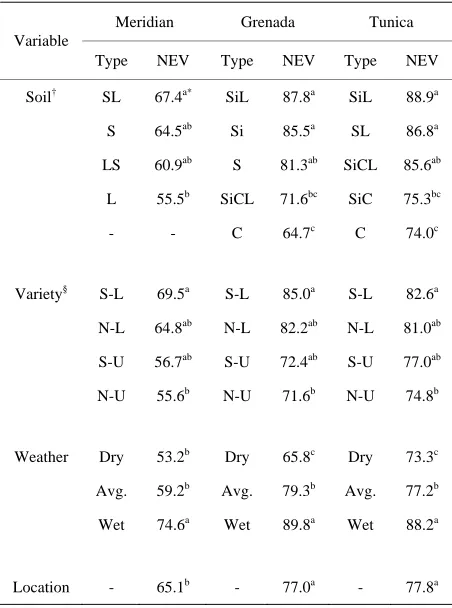
The results showed significant difference in the NEV as well as CCB of switchgrass-based ethanol production

among soils for all locations (Table 1). For a change

from one soil to another, values of these variables changed by 15% - 36%, depending on soil and location. In general, the values of NEV and CCB increased in the direction of heavier to lighter soils for all locations: clay

Figure 1. Simulated vs. observed switchgrass biomass yields (kg·ha–1) belonging to three varieties (Alamo, Cave-in-Rock, and Kanlow) for Starkville, MS, during 2001-2007. RMSE = root mean square error (kg·ha–1), d-ind = Willmott index, ME = modeling efficiency (Nash-Sutcliffe index), R2 = co- efficient of determination.

Table 1. The medians of net energy value (NEV: GJ·ha–1) asso- ciated with various soils, varieties, weather, and locations in Mississippi, USA.

Meridian Grenada Tunica Variable

Type NEV Type NEV Type NEV

Soil† _{SL 67.4}a* _{SiL 87.8}a _{SiL 88.9}a

S 64.5ab _{Si 85.5}a _{SL 86.8}a

LS 60.9ab _{S 81.3}ab _{SiCL 85.6}ab

L 55.5b _{SiCL 71.6}bc _{SiC 75.3}bc

- - C 64.7c _{C 74.0}c

Variety§ S-L 69.5a S-L 85.0a S-L 82.6a

N-L 64.8ab _{N-L 82.2}ab _{N-L 81.0}ab

S-U 56.7ab S-U 72.4ab S-U 77.0ab

N-U 55.6b _{N-U 71.6}b _{N-U 74.8}b

Weather Dry 53.2b _{Dry 65.8}c _{Dry 73.3}c

Avg. 59.2b _{Avg. 79.3}b _{Avg. 77.2}b

Wet 74.6a _{Wet 89.8}a _{Wet 88.2}a

Location - 65.1b - 77.0a - 77.8a

†

to silt loam for Tunica and Grenada and loam to sandy

loam for Meridian (Figure 2). For Tunica, the values of

NEV and CCB for loam soils were significantly higher than those for clay. Silty loam, sandy loam, and silty clay loam were not different, and neither were silty clay and clay. Silty clay was different from silty loam and sandy loam only. For Grenada, silty loam and silt had signifi- cantly higher values of NEV and CCB than silty clay loam and clay. Sand was different from only clay among the five soils. Silty clay loam was different from silty loam and silt but the same as sand and clay. For Meridian, only sandy loam values were significantly higher than those of loam. Sandy loam, sand, and loamy sand were about the same, and so were sand, loamy sand, and loam.

Figure 2. Net Energy Values (NEV) associated with various soils, weather conditions, and varieties for: (a) Tunica; (b) Grenada; and (c) Meridian in Mississippi.

The differences among the soils were likely due to varia- tions in their physical and chemical characteristics [36]. The establishment, growth, productivity, and survival of switchgrass were possibly affected by water holding ca- pacity, which is defined by soil texture [8]. Lighter soils with good water holding capacities and aeration pro- duced more biomass yields. The effect of soil on CCB

was the same as on NEV (Table 2) because these vari-

ables were linearly related: CCB = 0.1548NEV for Tu- nica, CCB = 0.1550NEV for Grenada, and CCB = 0.1556NEV for Meridian.

3.3. Variety Effect

In general, the values of NEV and CCB increased on the order of north-upland, south-upland, north-lowland, and

south-lowland varieties for all locations (Figure 2).

These results agree with those of Casler et al. [13]. They

observed the occurrence of similar pattern for the locations with latitudes of up to 40˚N, above which northlowland

Table 2. The medians of carbon credit balance (CCB: cred- its·ha–1) associated with various soils, varieties, weather, and locations in Mississippi, USA.

Meridian Grenada Tunica Variable

Type CCB Type CCB Type CCB

Soil† _{SL 10.5}a* _{SiL 13.6}a _{SiL 13.8}a

S 10.1ab _{Si 13.2}a _{SL 13.4}a

LS 9.5ab _{S 12.6}ab _{SiCL 13.2}ab

L 8.8b SiCL 11.4bc SiC 11.7bc

- - C 10.3c _{C 11.5}c

Variety§ _{S-L 10.8}a _{S-L 13.2}a _{S-L 12.8}a

N-L 10.1ab _{N-L 12.7}ab _{N-L 12.5}ab

S-U 8.9ab _{S-U 11.2}ab _{S-U 11.9}ab

N-U 8.1b _{N-U 11.1}b _{N-U 11.8}b

Weather Dry 8.3b _{Dry 10.2}c _{Dry 11.4}c

Avg. 9.2b Avg. 12.7b Avg. 12.0b

Wet 11.6a _{Wet 13.6}a _{Wet 13.6}a

Location - 10.2b _{- 11.9}a _{- 12.1}a

varieties produced the largest yields of all varieties. In our study, the proportion of increase from southupland to north-lowland, however, was larger than those from north-upland to south-upland and from north-lowland to south-lowland, indicating that the inter-cytotype (low- land vs. upland) difference is larger than the interecotype difference within the cytotype (north vs. south) in the southern region of United States. The differences among the varieties were because upland (lowland) cytotypes have preferential adaptation to northern (southern) lati- tudes [13]. That is, the yield advantage of a lowland (up- land) cytotype in a southern (northern) location is greater than in a northern (southern) location.

Although the NEV and CCB values followed the above pattern, only north-upland and south-lowland varieties were significantly different from each other for all loca-

tions (Tables 1 and 2). This difference was likely be-

cause these two varieties belonged not only to different cytotypes (upland vs. lowland) but also to different eco- types (north vs. south). The other pairs did not vary from one another because they belonged to either the same ecotype or the same cytotype. The varieties south-upland and north-lowland were also about the same because they belonged to the same origin (central Oklahoma), whereas south-lowland and north-upland were originated in the central/south Texas and central Great Plains, respectively

[14]. Several researchers, such as Sanderson et al. [5],

Casler [13], Parrish and Fike [8], and Stroup et al. [37],

found similar results. That is, upland cytotypes yielded substantially less than their lowland counterparts at all sites of their experiments. The larger yields in lowland cytotypes were because they are better adapted to the warmer and moister habitats of the southern region [4]. The poor performance of the upland cytotypes compared with their lowland counterparts in the southern region was due to their daylength sensitivity and early maturity [5]. The lowland varieties, on the other hand, matured later than their upland counterparts and thus produced larger yields [37]. The larger yields of the more southern locations were likely due to longer growing season and or warmer temperature. Switchgrass is highly photope- riod-sensitive. Moving upland (lowland) cytotypes south- ward (northward) speeds up (delays) their reproductive maturity, shortens (extends) their growing season, and thus reduces (increases) yields [13,38].

The differences among upland and lowland cytotypes were influenced by the type of year (dry or wet). Gaps between lowland and upland varieties were smaller in a

dry year than in a wet year for all locations (Figure 2).

These results agree with those of Wullschleger et al. [39],

in which differences between upland and lowland varie- ties were seasonally and environmentally dependent. In their study, upland varieties had shown less reduction in photosynthetic rates than their lowland counterparts in a

dry year. Also in the study of Stroup et al. [37], upland

varieties had exhibited less yield decrease than lowland ones under water stress conditions. This difference was because lowland cytotypes are associated with more hy- dric regions, whereas upland cytotypes are associated with more mesic regions. Upland cytotypes are more drought tolerant than their lowland counterparts [12,37].

3.4. Weather Effect

In general, the values of NEV and CCB increased on the order of dry year, average year, and wet year for all loca-

tions (Figure 2). These results were likely because wet

years produced more biomass yields and thus larger val- ues of these variables than did dry years. Under water stress conditions, switchgrass yielded less due to reduc- tion in photosynthetic rates and leaf water potential [37]. Accordingly, the NEV and CCB values in a wet year were significantly larger than those in a dry year for all

locations (Tables 1 and 2). The difference between an

average year and a dry or wet year, however, depended on location. For Grenada and Tunica, the average year was different from both wet and dry years, whereas it was about the same as dry year for Meridian. These dif- ferences were due to variation in precipitation distribu- tions during the growing seasons of switchgrass. The distribution of precipitation in Meridian in an average year was not very different from that in a dry year, whereas the precipitation distributions among the years

were different for the other two locations (Figure 3).

The differences between upland and lowland varieties

were larger in a wet year than in a dry year (Figure 2).

These results were similar to those of Sanderson et al. [5] and indicated that precipitation is a predominant factor affecting switchgrass productivity in southern locations. In their studies, the upland varieties from the U.S. Mid- west region had matured earlier and produced less bio- mass than the lowland varieties from the southern region. For lowland cytotypes, precipitation is the most impor- tant climate variable [40].

3.5. Location/Latitude Effect

Generally, values of both response variables increased in

the direction of south to north (Figure 2). The proportion

Figure 3. Precipitation distribution during switchgrass growing season in a: (a) dry year; (b) average year; and (c) wet year for Meridian; (d) dry year; (e) average year; and (f) wet year for Grenada; and (g) dry year; (h) average year; and (i) wet year for Tunica in Mississippi, USA.

The above differences among the locations were mainly due to variations in soil texture and precipitation. The ab-solute values of NEV and CCB, therefore, would not re-flect the effect of latitude, if any, on these variables. Thus, normalized values of these variables were used instead of absolute values to eliminate location effects (soil and weather), if any. The normalized value of a re- sponse

variable R for location L, denoted as NLR, was computed

as: NLR VRL LR L

V

L

N

[12].

,

where R is NEV or CCB, R is the value of R for loca-

tion L and variety V, and LR is the value of R for loca-

tion L. As the results showed, the R values for low-

land types decreased, whereas those for upland types in-

creased northwards (Figure 4). Thus, the differences

among the varieties increased southwards although only north-upland and south-lowland varieties were signifi- cantly different. The results were in agreement with those

of Casler et al. [13], who observed that upland (lowland)

cytotypes had preferential adaptation to northern (south- ern) latitudes. They found that north-upland cytotypes had steeper positive slopes than their south-upland counter- parts, whereas south-lowland cytotypes had steeper nega- tive slopes than their north-lowland counterparts. South- lowland cytotypes tend to produce more than north-up- land cytotypes in southern locations, whereas north-up- land cytotypes tend to have larger yields than south- lowland cytotypes in northern locations [5,13]. Whereas upland cytotypes are generally better adapted to well drained soils in higher latitudes, lowland cytotypes are typically adapted to moist locations in lower latitudes

Figure 4. The normalized values of Net Energy Value (NEV

4. Conclusion

nificant differences in NEV and CCB

increased for upland cytotypes.

) and carbon credit balance (CCB) belonging to four cytotypes for three locations in Mississippi, USA.

Results showed sig

5. Acknowledgements

work This material is based upon Sustainable Energy Research

performed through the Centre at Mississippi State

[1] E. Gnansouno no-Economic

lysis of Ligno view,” Bioresource

University and is supported by the Department of Energy under Award DE-FG3606GO86025.

REFERENCES

u and A. Dauriat, “Tech cellulosic Ethanol: A Re

Ana-

Technology, Vol. 101, No. 13, 2010, pp. 4980-4991. doi:10.1016/j.biortech.2010.02.009

[2] G. W. Huber and B. E. Dale, “Grassoline at the Pu Scientific American, Vol. 301, No. 1, 2

mp,” 009, pp. 52-59. doi:10.1038/scientificamerican0709-52

[3] J. Hill, E. Nelson, D. Tilman, S. Polasky and D. Tiffan “Environmental, Economic, and Energetic

y Costs and Be-

,

nefits of Biodiesel and Ethanol Biofuels,” Proceedings of the National Academy of Sciences of the United States of America, Vol. 103, No. 30, 2006, pp. 11206-11210. doi:10.1073/pnas.0604600103

[4] S. B. McLaughlin, J. Bouton, D. Bransby, B. V. Co W. R. Ocumpaugh, D. J. Parrish,

nger C. Taliaferro, K. P.

Vo-nt of Switchgrass for Biomass Feedstock and ,

gel and S. D. Wullschleger, “Developing Switchgrass as a Bioenergy Crop,” In: J. Janick, Ed., Perspectives on New Crops and New Uses, ASHS Press, Alexandria, 1999, pp. 282-299.

[5] M. A. Sanderson, J. C. Read and R. R. Reed, “Harvest Manageme

Forage Production,” Agronomy Journal, Vol. 91, No. 1, 1999, pp. 5-10.

doi:10.2134/agronj1999.00021962009100010002x [6] S. B. McLaughli

Ugarte, “Projecting Yield and Utilization Potentia n, J. R. Kiniry, C. M. Taliaferro and D. D.

l of Switchgrass as an Energy Crop,” Advances in Agronomy, Vol. 90, 2006, pp. 267-297.

doi:10.1016/S0065-2113(06)90007-8 [7] S. D. Wullschleger, E. B. D

Gunderson and L. R. Lynd, “Biomass P

avis, M. E. Borsuk, C. A roduction in

Swi-.

tchgrass across the United States: Database Description and Determinants of Yield,” Agronomy Journal, Vol. 102, No. 4, 2010, pp. 1158-1168.

doi:10.2134/agronj2010.0087 [8] D. J. Parrish and J. H. Fike, “

of Switchgrass for Biofuels,” C

The Biology and Agronomy ritical Reviews in Plant Sciences, Vol. 24, No. 5-6, 2005, pp. 423-459.

doi:10.1080/07352680500316433

[9] W. Zegada-Lizarazu, S. D. Wullschleger, S. S A. Monti, “Crop Physiology,” In: A

. Nair and . Monti, Ed., Switch- grass: A Valuable Biomass Crop for Energy, Springer- Verlag, London, 2012, pp. 55-86.

doi:10.1007/978-1-4471-2903-5_3 [10] J. R. Kiniry, C. R. Tischler and G.

diation Use Efficiency and Leaf CO

A. van Esbroeck,

“Ra-2 Exchange for

Di-verse C4 Grasses,” Biomass and Bioenergy, Vol. 17, No. 2, 1999, pp. 95-112. doi:10.1016/S0961-9534(99)00036-7 [11] S. Mani, L. G. Tabil and S. Sokhansanj, “Grinding Per-

formance and Physical Properties of Wheat and Barley

Straws, Corn Stover and Switchgrass,” Biomass and Bio- energy, Vol. 27, No. 4, 2004, pp. 339-352.

doi:10.1016/j.biombioe.2004.03.007

[12] C. L. Porter, “An Analysis of Variation between and Lowland Switchgrass, Panicum vir

Upland gatum L., in Cen- tral Oklahoma,” Ecology, Vol. 47, No. 6, 1966, pp. 980- 992. doi:10.2307/1935646

[13] M. D. Casler, K. P. Vogel, C. M. Taliaferro and R. L. Wynia, “Latitudinal Adaptation of Switchgrass Populations,” Crop

olf, C. Taliaf-Science, Vol. 44, No. 1, 2004, pp. 293-303.

[14] M. A. Sanderson, R. L. Reed, S. McLaughlin, S. D. Wull-schleger, B. V. Conger, D. J. Parrish, D. D. W

erro, A. A. Hopkins, W. R. Ocumpaugh, M. A. Hussey, J. C. Read and C. R. Tischler, “Switchgrass as a Sustainable Bio-energy Crop,” Bioresource Technology, Vol. 56, No. 1, 1996, pp. 83-93.

doi:10.1016/0960-8524(95)00176-X

[15] N. Di Virgilio, A. Monti and G. Venturi, “Spatial Var ability of Switchgrass (Panicum virga

i- tum L.) Yield as Related to Soil Parameters in a Small Field,” Field Crops Research, Vol. 101, No. 2, 2007, pp. 232-239.

doi:10.1016/j.fcr.2006.11.009

[16] T. Persson, A. Garcia, Y. Garcia, J. O. Paz, J and G. Hoogenboom, “Maize Et

. W. Jones hanol Feedstock Produc- tion and Net Energy Value as Affected by Climate Vari- ability and Crop Management Practices,” Agricultural Systems, Vol. 100, No. 1-3, 2009, pp. 11-21.

doi:10.1016/j.agsy.2008.11.004

[17] H. M. Benedict, “Effect of Day Length and Tempe the Flowering and Growth of Fou

rature on r species of Gras- ses,”

om, “Determining the Impact of Climate and Journal of Agricultural Research, Vol. 61, No. 9, 1940, pp. 661-672.

[18] T. Persson, B. V. Ortiz, D. I. Bransby, W. Wu and G. Hoogenbo

Soil Variability on Switchgrass (Panicum virgatum L.) Production in the South-Eastern USA: A Simulation Stu- dy,” Biofuels, Bioproducts and Biorefining, Vol. 5, No. 5, 2011, pp. 505-518. doi:10.1002/bbb.288

[19] S. B. McLaughlin and L. A. Kszos, “Development of Switchgrass (Panicum virgatum) as a Bioenergy Feed-stock in the United States,” Biomass and Bioenergy, Vol. 28, No. 6, 2005, pp. 515-535.

doi:10.1016/j.biombioe.2004.05.006 [20] S. Sokhansanj, A. Kumar and A. F. T

opment and Implementation of Integrat

urhollow, “Devel-ed Biomass Sup-ply Analysis and Logistics model (IBSAL),” Biomass and Bioenergy, Vol. 30, No. 10, 2006, pp. 838-847.

doi:10.1016/j.biombioe.2006.04.004

[21] J. R. Kiniry, J. R. Williams, P. W. Gassman an baeke, “A General, Process-Oriented Mo

d P. De-del for Two Com-

, R. L. Reed, M. A. Sanderson, peting Plant Species,” Transactions of the ASAE, Vol. 35, No. 3, 1992, pp. 801-810.

[22] J. R. Kiniry, K. A. Cassida, M. A. Hussey, J. P. Muir, W. R. Ocumpaugh, J. C. Read

V. Bridgewater and B. D. G. Bo

outheastern [23] J. R. Kiniry, L. Lynd, N. Greene, M. V. Johnson, M.

Casler and M. S. Laser, “Biofuels and Water Use: Com- parison of Maize and Switchgrass and General Perspec- tives,” In: J. H. Wright and D. A. Evans, Eds., New Re- search on Biofuels, Nova Science Publishers, Hauppauge, 2008, pp. 17-30.

[24] S. Sokhansanj and S. Mani, “Modeling of Biomass Supply

Logistics,” In: A. bcock,

Eds., Science in Thermal and Chemical Biomass Conversion, CPL Press, Newbury Perks, 2006, pp. 387- 403.

[25] P. Woli and J. O. Paz, “Evaluation of Various Methods for Estimating Global Solar Radiation in the S

USA,” Journal of Applied Meteorology and Climatology, Vol. 51, No. 5, 2012, pp. 972-985.

doi:10.1175/JAMC-D-11-0141.1 [26] P. I. R. Adler, M. A. Sanderson, A. A

and H. J. G. Jung, “Biomass Yield a

. Boateng, P. J. Weimer nd Biofuel Quality of Switchgrass Harvested in Fall or Spring,” Agronomy Journal, Vol. 98, No. 6, 2006, pp. 1518-1525.

doi:10.2134/agronj2005.0351 [27] S. Hwang, F. M. Epplin, B. Lee and

babilistic Estimate of the Freque

R. Huhnke, “A Pro-ncy of Mowing and Bal-ing Days Available in Oklahoma USA for the Harvest of Switchgrass for Use in Biorefineries,” Biomass and Bio- energy, Vol. 33, No. 8, 2009, pp. 1037-1045.

doi:10.1016/j.biombioe.2009.03.003

[28] A. Kumar and S. Sokhansanj, “Switchgrass (Panicum vi-gratum L.) Delivery to a Biorefinery Using Integrated Biomass Supply Analysis and Logistics (IBSAL) Model,” Bioresource Technology, Vol. 98, No. 5, 2007, pp. 1033- 1044. doi:10.1016/j.biortech.2006.04.027

[29] S. Sokhansanj, S. Mani, A. Turhollow, A. Kumar, D. Bransby, L. Lynd and M. Laser, “Large-Scale Production, Harvest and Logistics of Switchgrass (Panicum virgatum L.)—Current Technology and Envisioning a Mature Tech- nology,” Biofuels, Bioproducts and Biorefining, Vol. 3, No. 2, 2009, pp. 124-141. doi:10.1002/bbb.129

[30] R. Mitchell, K. P. Vogel and D. R. Uden, “The Feasibility of Switchgrass for Biofuel Production,” Biofuels, Vol. 3, No. 1, 2012, pp. 47-59. doi:10.4155/bfs.11.153

[31] M. R. Schmer, K. P. Vogel, R. B. Mitchell and R. K. Per- rin, “Net Energy of Cellulosic Ethanol from Switchgrass,” Proceedings of the National Academy of Sciences of the USA, Vol. 105, No. 2, 2008, pp. 464-469.

doi:10.1073/pnas.0704767105

[32] L. Luo, E. van der Voet and G. Huppes, “Energy and En- vironmental Performance of Bioethanol from Different Lignocelluloses,” International Journal of Chemical En- gineering, Vol. 1-12, 2010, pp. 1-12.

doi:10.1155/2010/740962

[33] X. Qin, T. Mohan, M. El-Halwagi, G. Cornforth and B. A. McCarl, “Switchgrass as an Alternate Feedstock for Pow- er Generation: An Integrated Environmental, Energy and Economic Life-Cycle Assessment,” Clean Technologies and Environmental Policy, Vol. 8, No. 4, 2006, pp. 233- 249. doi:10.1007/s10098-006-0065-4

[34] M. Wang, Y. Wu and A. Elgowainy, “Operating Manual

ycle As- for GREET: Version 1.7,” Argonne National Laboratory, Argonne, 2007.

www.transportation.anl.gov/pdfs/TA/353.pdf.

[35] S. Spatari, Y. Zhang and H. L. Maclean, “Life C sessment of Switchgrass- and Corn Stover-Derived Etha- nol-Fueled Automobiles,” Environmental Science and Technology, Vol. 39, No. 24, 2005, pp. 9750-9758. doi:10.1021/es048293

[36] W. L. Stout, “Water-Use Efficiency of Grasses as Affected by Soil, Nitrogen, and Temperature,” Soil Science Society of America Journal, Vol. 56, No. 3, 1992, pp. 897-902. doi:10.2136/sssaj1992.03615995005600030036x [37] J. A. Stroup, M. A. Sanderson, J. P. Muir, M. J. Mc-

Farland and R. L. Reed, “Comparison of Growth and Per- formance in Upland and Lowland Switchgrass Types to Water and Nitrogen Stress,” Bioresource Technology, Vol. 86, No. 1, 2003, pp. 65-72.

doi:10.1016/S0960-8524(02)00102-5

[38] M. A. Sanderson and D. D. Wolf, “Morphological Deve- lopment of Switchgrass in Diverse Environments,” Agro- nomy Journal, Vol. 87, No. 5, 1995, pp. 908-915. doi:10.2134/agronj1995.00021962008700050022x [39] S. D. Wullschleger, M. A. Sanderson, S. B. McLaughlin,

D. P. Biradar and A. L. Rayburn, “Photosynthetic Rates and Ploidy Levels among Populations of Switchgrass,” Crop Science, Vol. 36, No. 2, 1996, pp. 306-312.

doi:10.2135/cropsci1996.0011183X003600020016x [40] M. G. Tulbure, M. C. Wimberly, A. Boe and V. N. O-