Munich Personal RePEc Archive
Sanitation and Hygiene
Borooah, Vani
University of Ulster
May 2018
Online at
https://mpra.ub.uni-muenchen.de/90420/
1
Chapter 4: Sanitation and Hygiene
1. Introduction
It is universally accepted that poor sanitation and hygiene are a major cause of disease in
developing countries. In India, poor sanitation takes the form of an absence of toilets in households’
dwellings which ipso facto compel their members to defecate in the open. This practice spreads
bacterial infections like diarrhoea, cholera, and hook worm which, in turn, have repercussions on
child development (Coffey et. al. 2017, Spears, 2013, Chambers and von Medeazza, 2013, Ghosh, et.
al. 2014). Poor hygiene, particularly the failure of mothers to wash hands after defecation, is a prime
cause of diarrhoea in children in developing countries. The vast majority of diarrhoeas are caused by
infectious pathogens which reside in faeces and which employ a variety of routes to enter a new host.
Since one such route is getting onto fingers and, thereby, into foods and fluids the incidence of
diarrhoea can be reduced by improvements in domestic hygiene1 Given that diarrhoea accounts for
1.8 million deaths in children in low and middle income countries it is important to examine hand
washing practices (Borooah, 2004; Huang and Zhou, 2007, Ejemot-Nwadiaro et. al., 2015 ).
Against this background, this paper examines, within the Indian context, patterns of toilet use
and personal hygiene. Open defecation in India has attracted a great deal of academic interest and its
eventual elimination, through a program of building toilets, has been an important object of
successive Indian governments from the Total Sanitation Campaign, the Nirmal Bharat Abhiyan, and
the Swach Bharat Abhiyan.2 An important and influential line in academic thinking, as articulated in
Coffey and Spears (2017) and Coffey et. al. (2017), is that “widespread open defecation in rural India
is not attributable to relative material or educational deprivation but rather to beliefs, values, and
norms about purity, pollution, caste and untouchability … that cause people to consider having and
using a pit latrine as ritually impure and polluting. Open defecation, in contrast, is seen as promoting
1
This is particularly important in India where children are fed by hand. 2
2
purity and strength, particularly by men” (Coffey et. al. 2017, p. 59).3 So, on this analysis, persons in
rural India have an aversion to affordable toilets (of the pit latrine type) while simultaneously having
a preference for open defecation.4
A combination of aversion and preference then is the prime reason, as the Planning
Commission (2013) found, why in 73% of households in rural India at least one person practiced open
defecation but the members of 66% of households had no option but to defecate in the open because
their dwellings lacked toilets. So, while there might be some mild preference for open defecation – in
the sense that some members of households that had toilets nevertheless defecated in the open – the
root cause of open defecation was a lack of toilets.
The contribution of this paper is that it examines both toilet possession and personal hygiene
in India. It shows that the strongest influences on households in India having a toilet were their
standard of living, the highest educational level of adults in the households, and whether or not they
possesses ancillary amenities like a separate kitchen for cooking, a pucca roof and floor, and water
supply within the dwelling or its compound. However, in so doing, it also shows that whether
households had toilets depended not just on household-specific factors but also on the social
environment within which the households were located. More specifically, ceteris paribus households
in more developed villages would be more likely to have a toilet than those in less developed villages.
The effect of households’ social environment on their “consumption” of toilets in developing
countries is termed in this paper - in homage to Duesenberry (1967) who, through his “demonstration
effect” first drew attention to the influence on consumers, when making consumption decisions, of
their social context - as the “developmental demonstration” effect.5 Duesenberry (1967) maintained
that a person’s success and self-esteem was defined in terms of the acquisition of material goods and,
so, in order to avoid a loss of self-esteem, an individual would try to “keep up with the Joneses”.
Thus, as McCormick (1983) writes, “frequent exposure to higher quality goods than one usually
3
Coffey et. al. (2017) also claim that rural women prefer open defecation to using a household toilet because it gives them an opportunity to escape, however temporarily, the confines of their homes.
4
Another source of aversion to pit latrines is anxiety about having them emptied. 5
3
consumes will cause an increase in one’s consumer expenditure” (p.1126). Duesenberry (1967)
labelled this the “demonstration effect” (p.27).
However, the relentless march of neo-classical economics in the 1930s and 1940s,
culminating with the publication of Paul Samuelson’s Foundations of Economic Analysis in 1947)
meant that all reference to inter-dependent consumers preferences, engendered by social interactions,
were expunged from economics thereby reducing consumers to what Sen (1977) described as
“rational fools”.6 This paper attempts to escape this neo-classical paradigm of a consumer oblivious
of his/her social by formulating, and testing, a model in which households’ demand for toilets in rural
India varies according to the level of development of the villages in which they reside.
Jenkins and Curtis (2005) examined the motives for acquiring a latrine in Benin in terms of
“desires for change arising out of dissatisfaction from a perceived difference between a desired or an
ideal state and one’s actual state or situation” (p.2447).7 They found that the demand for toilets in
rural Benin had less to do with a desire for a healthier environment and much more to do with the
prestige and status that latrine ownership implied in terms of an urbanised modern style of living.8 It
was dissonance between what one had and, given the social context, what one thought one ought to
have, that generated demand for toilets rural Benin.
These findings were echoed by Rosenboom’s et. al. (2011) study of the demand for toilets in
Cambodia. They found that there was a strong perception among rural Cambodians about the ‘ideal’
latrine consisting “of a pour-flush pan and solid walls and roof …with respondents expressing
reluctance to purchase anything less than the ideal latrine preferring to wait until they could afford a
better model” (p.24). Of the two types of toilet - the traditional pit latrine9 or the flush (pour-flush or
fully flushable) - by far the most common in India was the flush toilet: 64% of rural households had a
toilet of this type compared to 36% that had a pit latrine.10 So, it is likely that rural Indians prefer a
6
See (Mason, 2000). 7
See Bagozzi and Lee (1999) 8
See Cairncross (2003). 9
Given the cost of building sewers and sewage treatment plants, a common form of latrine in rural India are pit latrines which store faeces underground. Under WHO guidelines of a pit of around 60 cubic feet, a latrine pit is expected to fill up after approximately five years if used daily by a family two adults and four children after which it must be emptied or a new pit built (Coffey et. al. (2017).
10
4
certain type of toilet and are prepared to wait until these can be afforded: the “preference for open
defecation” that, according to Coffey et. al. (2017), exists among rural Indians may be nothing more
than a willingness to wait until the right type of toilet could be bought.
Lastly, the paper considers the issue of personal hygiene, in particular, whether people
washed their hands after defecation and, if they did, what they washed their hands with. The raw data
show a greater ownership of toilets by Muslim, relative to Hindu, households but they also show that
Hindus have a greater sense of personal hygiene, defined as post-defecation hand washing with soap,
than Muslims. All these “facts” should, however, be treated with caution: Hindus and Muslims differ
in more aspects than just religion and the question is whether their differences, in terms of toilet
ownership and hygiene, survive after these non-religion variables have been controlled for. This paper
imposes these controls and, in so doing, suggests that these differences between households from the
two groups are not as stark as some people might like to believe.
The results reported in this paper should, however, be prefaced with some clarificatory
remarks. The paper’s analysis pertains to households and not to persons within them. Estimating the
number of persons defecating in the open by computing the number of persons in households without
a toilet would almost certainly be an underestimate since some persons from households with a toilet
also defecated in the open. The Planning Commission’s (2013) estimate was that of 100 rural persons,
73 defecated in the open and of these 66 were from households without a toilet; consequently, 7
persons, out of the 73 who defecated openly, (or 10%) did so in spite of living in houses with a toilet.
Similarly, the data on handwashing analysed in the paper related to households with the implicit
assumption being that, depending on a household’s response, every member within it washed, or did
not wash, their hands after defecation. Needless to say, this, too, will not always be true.
The results reported in this chapter are from the India Human Development Survey (hereafter,
IHDS-2011) which relates to the period 2011-12.11 This is a nationally representative, multi-topic
panel survey of 42,152 households in 384 districts, 1420 villages and 1042 urban neighbourhoods
across India. Each household in the IHDS-2011 was the subject of two hour-long interviews. These
interviews covered inter alia issues of: health, education, employment, economic status, marriage,
11
5
fertility, gender relations, and social capital. The IHDS-2011, like its predecessors for 2005 and 1994,
was designed to complement existing Indian surveys by bringing together a wide range of topics in a
single survey. This breadth permits the analysis of associations across a range of social and economic
conditions.
2. A Preliminary Look at the Data
Of particular relevance to this study is that the IHDS-2011 reported on each household’s
housing conditions: inter alia whether the dwelling had a toilet and, if it did, what type of toilet12;
whether it had a separate kitchen; whether it had a separate vent in the cooking area; whether the
household had electricity; whether the household’s water supply was within the dwelling or its
compound; the nature of the dwelling’s roof and floor.13 Since the concern of this chapter is with
open defecation, a small number of households (for example, living in chawls) that did not have
toilets in their homes, but had access to communal or public toilets, were excluded from the analysis.
After this exclusion it could be inferred that members of households that did not have a toilet would
perforce have to defecate in the open.14
<Table 1>
Table 1 reports that of the total of households in the IHDS-2011: 52.6% had a toilet; 54.9%
had a separate kitchen; 50.6% had their water supply within the dwelling; 64.3% had a pucca roof ;
and 59.3% had a pucca floor.15 These figures, however, mask a rural-urban divide. In the less
developed villages, only 31.1% of households had a toilet and this rose to 45.2% of households in
more developed villages. By contrast, 96.6% of households in metropolitan areas, and 83.5% of
households in non-metropolitan urban areas, had a toilet within their homes.
12
These were: traditional pit latrines; semi-flush toilets connected to septic tank; flush toilets. 13
The roof and floor could be: ‘kutcha’ (grass, mud, thatch, wood, tile, slate for the roof; mud or wood for the floor); or ‘pucca’ (asbestos, metal, brick, stone, concrete for the roof; brick, stone, cement, tiles for the floor). 14
Since some members of households with a toilet might also prefer to defecate in the open this is likely to be an underestimate of the number of persons practicing open defecation.
15
6
For this reason, the analysis of the prevalence of toilets within the household dwelling
reported in this paper is restricted to rural households.16 Table 1 shows that, of rural households, the
‘Other’ social group, comprising Christians, Sikhs, and Jains, were most likely to have a toilet (and
also amenities like a separate kitchen, water supply within their dwellings, and pucca roofs and floors)
while the Scheduled Castes (SC) and Scheduled Tribes (ST) were least likely to have a toilet (only
27.2% of SC and 26.5% of ST households had a toilet) and other ancillary amenities.
<Figures 1 and 2>
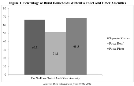
Figure 1 shows the amenities in the homes of rural households that did not have a toilet: two
in three rural households that did not have a toilet, did not also have a separate kitchen; one in two
households that did not have a toilet, did not also have a pucca roof; and over two-thirds of
households that did not have a toilet, did not also have a pucca floor. Thus a majority of households
that could not afford a toilet could not also afford ancillary amenities like a separate kitchen or a
pucca roof or floor.
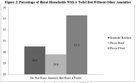
Figure 2 shows the dwelling amenities of rural households that did have a toilet: only 30% of
households that had a toilet did not have a separate kitchen or a pucca roof and one-third of
households that had a toilet did not have a pucca floor. Thus only a minority of households that had a
toilet did not have ancillary amenities like a separate kitchen or a pucca roof or floor.
3. Specifying the Demand for Toilets Equation
In estimating the demand for toilets in India, the dependent variable yi, defined over N
households (indexed, i=1…N), was assumed to take the value 1 if household i had a toilet (in its
dwelling) and 0 if it did not.17 It should be emphasised that in estimating the logit model, it was not
possible, for reasons of multicollinearity, to include all the categories with respect to the variables: the
category that was omitted for a variable is referred to as the reference category (for that variable).
16
That is households living in ‘less’ or ‘more’ developed villages. After grossing up, these comprised 68.7% of the households in IHDS-2011with 39.4% and 29.3% of all households living in, respectively, ‘less’ and ‘more’ developed villages.
17
7
If Pr[yi=1] and Pr[yi=0] represent, respectively, the probabilities of a household having and
not having a toilet, the logit formulation expresses the log of the odds ratio as a linear function of K
variables (indexed k=1…K) which take values, X Xi1, i2...XiK with respect to household i, i=1…N:
1
Pr[ 1]
log
1 Pr[ 1]
K i
k ik i i k
i y
X u Z
y = β
=
= + =
− =
∑
(1)
where: βk is the coefficient associated with variable k, k=1…K.
From equation (1) it follows that:
ˆ ˆ 1 Pr[ 1] 1 i i i i z X
i z X
e e e y e β β + = = =
+
(2)
where, the term ‘e’, in the above equation represents the exponential term.
The variables used to explain the demand for toilets were grouped as follows:
A. Social Group.
These related to the social group, defined in terms of religion/caste, to which the households
belonged: Brahmins; Forward Caste Hindus (FCH); Hindus from the Other Backward Classes (OBC),
Scheduled Castes (SC); Scheduled Tribes (ST); Muslims; and an ‘Other’ category comprising
Christians, Sikhs, and Jains.
A great deal has been made recently about the propensity of households from different social
groups to have toilets. Coffey and Spears (2017) argue that Muslim households were more likely to
have a latrine, even it was a rudimentary one, than Hindus and they ascribed this to Hindus facing the
religious constraints of ritual pollution so that the presence of a toilet within the Hindu home was
regarded as impure and unclean. They went on to attribute the lower infant and child mortality among
Muslims vis-à-vis Hindus18 to the lower propensity of Muslims, compared to Hindus, to defecate in
the open: Muslim neighbourhoods would be less susceptible to the spread of infections caused by the
greater likelihood contact with faecal matter under open defecation. However, over a decade earlier,
Borooah and Iyer (2005) had pointed out that the lower infant mortality among Muslims was confined
to the girl child with Muslim-Hindu infant mortality rates for boys being broadly similar and this was
18
8
because while Hindus and Muslims had the same degree of “son preference” Hindus had a higher
degree of “daughter aversion”.
B. Income and Education.
It might be expected that a household’s demand for a toilet in the home, like the demand for
any commodity, would be affected by is income. To capture the “income effect” each household was
placed in one of five quintiles of household per capita consumption (lowest, 2nd quintile, 3rd quintile,
4th quintile, highest quintile) depending upon its reported per-capita consumption.
It might also be expected that higher the educational level of a household’s members the
lower would its members’ propensity to defecate in the open: higher levels of education would lead to
greater awareness of the health hazards of open defecation; additionally, higher levels of education
might be associated with a greater sense of the social impropriety of open defecation. The education
level of a household was captured by the highest level of education of an adult member. Five levels of
education were distinguished: (i) no education; (ii) up to primary level of schooling; (iii) above
primary and up to secondary level of schooling; (iv) higher secondary; (v) graduate or above.
C. Region
The incidence of open defection (through not having a toilet in in the house) also varies
according to the culture of a region. A district level map of the proportion of persons defecating in
the open (Coffey et. al., 2014) shows a high incidence of open defecation in the central and southern
states, with a comparatively low incidence in the eastern and western states, of India. Open defecation
was particularly common in four states of the “Hindi heartland” - Bihar, Madhya Pradesh, Rajasthan,
Uttar Pradesh – with 82.4% and 78.2% and of rural households in Bihar and Uttar Pradesh not having
a toilet; by contrast, in the north-eastern states of Mizoram and Manipur, only 14% and 15.4%,
respectively, of rural households did not own a toilet (Coffey and Spears, 2017).
In order to capture this regional dimension to open defecation (or more precisely, household
non-ownership of toilets) this study aggregated the Indian states into the following regions: North
(comprising the states of Jammu & Kashmir, Delhi, Haryana, Himachal Pradesh, Punjab (including
Chandigarh), and Uttarakhand); the Centre (Bihar, Chhattisgarh, Madhya Pradesh, Jharkhand,
9
states19); the West (Gujarat and Maharashtra); and the South (Andhra Pradesh, Karnataka, Kerala, and
Tamil Nadu).
D. Other Housing Amenities
Figures 1 and 2 showed a strong association between households having a toilet in the
dwelling and also having other amenities like a separate kitchen, pucca roof and floor, and water
supply within the house or its compound. So, the other set of variables included in the equation were
the presence or absence of these “non-toilet” amenities, the hypothesis being that a household was
more likely to have a toilet if it already had a separate kitchen or pucca roof or floor or its water
supply within the house and ipso facto less likely to have toilet if it did not have one or more of these
amenities.
E. Households Practicing Untouchability
A recurring view on open defecation (Cofey et. al. 2014; Cofey and Spears, 2017; Coffey et.
al. 2017; Spears and Thorat, 2015 )is that people living in rural India are reluctant to have pit latrines
in their home because they regard them as dirty and, in particular, are alarmed by the prospect of
facing, after the toilet has been used for a certain period, the unpleasant task of emptying the pit: this
they are not prepared to do themselves; nor are they prepared to pay the high charges of having it
done by others.20
A way of testing this hypothesis is to examine whether the fact that some member of a
household practices untouchability impacts significantly on the propensity of that household to
possess a toilet. In the course of the IHDS-2011 interviews, each household was asked if “in your
household, do some members practice untouchability?” Although the IHDS did not explicitly define
what it regarded as ‘practicing untouchability’ it is reasonable to interpret this to mean the range of
measures used in order to avoid proximity with persons who, for reasons of ritual pollution, were
permanently ‘unclean’. 21 This ‘untouchability’ variable – which took the value 1 if a household’s
19
Sikkim, Arunachal Pradesh, Nagaland, Mizoram, Manipur, Tripura, Meghalaya. 20
Coffey et. al. (2017) quote ₹700-1,000 as the price of emptying a pit (which takes no more than a few hours) in rural Bihar where the daily wage does not exceed ₹200.
21
10
answer to the above question was ‘yes’ and 0 if its answer was ‘no’ – was, following Spears and
Thorat (2015),the included in the equation as an explanatory variable.
F. The Developmental Demonstration Effect
The hypothesis lying at the heart of this paper is the ‘developmental effect’ whereby the rising
tide of economic development lifts all boats and induces households to improve their dwelling’s
amenities by building kitchens, reinforcing their roofs and floors, improving their water supply and,
yes, by installing toilets. As discussed in the introductory section, this idea derives from Duesenberry
(1967) who argued that consumer demand could, and would, often be determined by social needs and
the aspirations of individuals.
Since increased consumption expenditures arise to “eliminate the feelings of inferiority
created by other people consuming superior goods” (McCormick, 1983, p. 1126), “inferiority feeling”
and “superior goods” would depend upon the social and cultural environment of consumers. In the
context of this paper, the lack of a toilet would not generate feelings of inferiority in a less developed
village in which relatively few people had a toilet and open defecation was the norm; however, the
same lack in a more developed village, in which several households had toilets, would generate a
sense of inadequacy in those households that did not possess a toilet and would propel these towards
building toilets for themselves. We label the demand for toilets emanating from this source as the
“developmental demonstration effect” (DDE).
On the basis of their respective infrastructure, the IHDS-11 separated villages into two types:
“less developed” villages (LDV) and “more developed” villages (MDV) with 57% of rural households
living in the LDV and 43% living in the MDV.22 The hypothesis of this study is that the operation of
the DDE systematically raised the demand for toilets in the MDV vis-à-vis the LDV. By this is meant
that the operation of the DDE affected each of variables under A-F in such a way that the likelihood
of having a toilet would, for a given value of a variable, be greater in a MDV than in a LDV. So,
worship – a plate, tumbler, kitchen utensil, the kitchen, the prayer room – which was touched by an
‘untouchable’ was instantly defiled and would have to be purified through ritual ablutions. 22
11
households in which the highest level of education of an adult was, say, higher secondary would
ceteris paribus be more likely to have a toilet in a MDV than in a LDV; households which were, say,
in the highest quintile of consumption would ceteris paribus be more likely to possess a toilet in a
MDV than in a LDV.
In order to test this hypothesis, the variable Vi, defined over all rural households indexed by i,
was assumed to take the value 1if a household lived in a MDV and 0 if it lived in a LDV. The
variable Vi was then allowed to interact with all the other variables so that the equation that was
estimated was:
1 1
Pr[ 1]
log ( )
1 Pr[ 1]
K K
i
k ik k ik i i i
k k
i y
X X V u Z
y = β = α
=
= + × + =
− =
∑
∑
(3)
Equation (3) shows that that the coefficient associated with variable k in the context of a
MDV (that is, Vi =1) is (βk +αk)while the coefficient associated with the same variable in the
context of a LDV (that is, Vi =0) isβk: consequently, in terms of the estimated coefficients, αk
represents variable k’s associated DDE from a “less developed” to a “more developed” village.
However, the logit estimates shown in equations (1) and (3) themselves do not have a natural
interpretation – they exist mainly as a basis for computing more meaningful statistics and the most
useful of these are the predicted probabilities (of having a toilet) defined by equation (2).23
Consequently, as suggested by Long and Freese (2014), the results from estimating equation (3) are
presented in Table 1 in the form of the predicted probabilities from the estimated logit coefficients of
the equation.
The Method of Recycled Predictions
The predicted probabilities were computed the method “recycled predictions” as described in
Long and Freese (2014, ch. 4) and in the Stata manual.24 Since this method underpins the results
presented in this paper it is useful, at the very outset, to describe it in some detail. The variable yi in
equation (1) is defined over households distinguished by different characteristics – by social group,
23
It should be noted that, by equation (3), the Zi in equation (2) differ according to whether the household’s village is a LDV or a MDV.
24
12
education, region etc. Suppose that one of these characteristics is religion and households are
identified, inter alia, by whether they are Hindu, Muslim, or Christian. The object is to identify the
predicted probabilities of having a toilet which can be entirely ascribed to religion and, further, to test
whether these differ significantly between the religions. The method of “recycled predictions” enables
one to do so.
Suppose that the first variable relates to households’ reigion so that Xi1=1 if household i is
Hindu, Xi1=2 if it is Muslim; Xi1=3 if it is Christian. For ease of exposition assume that the
households are ordered so that Xi1=1 for i=1…L and Xi1=2 for i=L+1…M and Xi1=3 for i=M+1…N .
Now, using the logit estimates from equation (1), equation (2) predicts for each household its
probability of having a toilet, denoted ˆp ii( =1... )N . The mean of the ˆpidefined over all the N
households in the estimation sample will be the same as the (estimation) sample proportion of
households that have toilets. Similarly, the mean of the ˆpidefined over the L Hindu (or, M-L Muslim,
or N-M Christian) households will be the same as the (estimation) sample proportion of Hindu (or
Muslim or Christian) households that have toilets. In other words, the estimated logit equation passes
through the sample means.25
However, the difference between the three sample means – Hindu ( ˆH
p ), Muslims ( ˆM p ), and
Christians ( ˆC
p ) – does not reflect the differences, due to solely to religion, between households in the
three groups in their probabilities of having a toilet. This is because the three groups differ not just in
terms of religion but also with respect to variables like income, education etc. Computing the mean
probabilities over each subgroup will not neutralise these differences and, hence, differences between
ˆH, ˆM, and ˆC
p p p cannot be attributed solely – though, of course, some part may be - to differences in
religion.
The method of “recycled predictions” isolates the effect on the predicted probability (of
having a toilet) of households belonging to different religions. First, “pretend” that all the households,
in the entire sample of N households are Hindu. Holding the values of the other variables constant
25
13
(either to their observed sample values, as in this paper, or to their mean values), compute the average
probability (of having a toilet) under this assumption and denote it H
p . Next, “pretend” that all the
households, in the entire sample of N households are Muslim and, again holding the values of the
other variables constant, compute the average probability (of having a toilet) under this assumption
and denote itpM.
Since the values of the non-religion variables are unchanged between these two hypothetical
scenarios, the only difference between them is that, in the first scenario, the Hindu variable is
“switched on” (with the Muslim and Christian variables “switched off”) - while , in the other, the
Muslim variable is “switched on” (with the Hindu and Christian variables “switched off”) - for all
households. 26 Consequently, the difference between H
p and M
p is entirely due to differences in
religion between Hindus and Muslims. In essence, therefore, in evaluating the effect of two
characteristics X and Y on the likelihood of a particular outcome, the method of “recycled predictions”
compares the two probabilities, first, under an “all have the characteristic X” scenario and, then, under
an “all have the characteristic Y” scenario – the values of the other variables unchanged between the
scenarios. The difference in the two probabilities is then entirely due to the attribute represented by X
and Y (in this case, differences in religion, more specifically, differences in between Hindus and
Muslims).27
4. Measuring the Development Demonstration Effect
In order to pass judgement on the existence (or otherwise) of the ‘development demonstration
effect’ (DDE), the predicted probability of having a toilet (hereafter, abbreviated to PPT) was
computed separately, with respect to every determining variable noted under A-F above, for
households in the LDV and the MDV; the difference in these PPT were then tested to see if they were
statistically significant: if the PPT with respect to a variable was ceteris paribus significantly higher in
26
In operational terms, these hypothetical scenarios are constructed in STATA by estimating the logit equation and then using the predict command after the command “replace Xi1=1” has been executed,: the average of these predictions over the N households will yieldpH; next, use the predict command after the command “replace Xi1=2” has been executed: the average of these predictions over the N households will yield
M p . In practice, STATA’s margin command will perform these calculations.
27
14
the MDV than in the LDV then that would be evidence of the presence of a DDE with respect to that
variable; conversely, the absence of a significantly different PPT between households in the MDV
vis-à-vis households in the LDV would be evidence that the DDE did not exist with respect to that
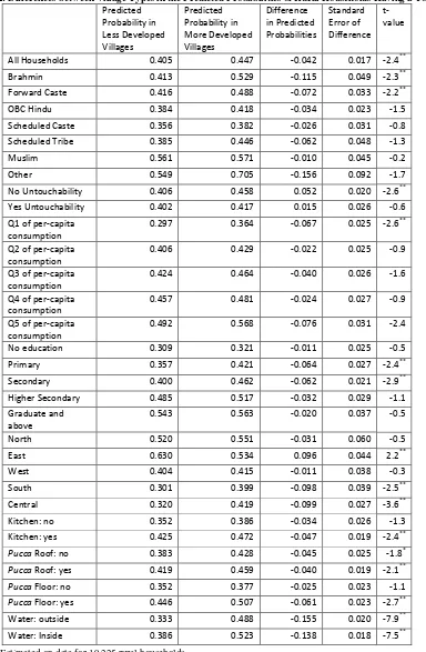
variable. These inter-village type PPT are shown in Table 2.
<Table 2>
The second and third columns of Table 2 show these probabilities for, respectively, the LDV
and the MDV. The PPT against the ‘All Households’ row and the “Less Developed Villages” column
were computed using the method of “recycled predictions”, discussed above, by assuming all the
19,225 households in the estimation sample lived in LDV or, in other words, by the applying the
coefficients relevant to the LDV (that is, the βk of equation (3)) to all the 19,225 households in the
estimation sample and computing the average likelihood of households having a toilet under this
‘all-LDV’ scenario.28 This yielded a PPT of 40.5%.
Similarly, the PPT against the ‘All Households’ row and the “More Developed Villages”
column were computed by assuming all the 19,225 households in the estimation sample lived in MDV
or, in other words, by the applying the coefficients relevant to the MDV (that is, the βk + αk of
equation (3)) to all the 19,225 households in the estimation sample and computing the average
likelihood of households having a toilet under this ‘all-MDV’ scenario. This yielded a PPT of 44.7%.
The difference in the LDV and MDV probabilities was -4.2 points (column 4).
Dividing this difference by its standard error (column 5) yielded a t-value of 2.4: the
observed difference of 4.2 points was, thus, significantly different from zero in the sense that the
likelihood of observing this value, under the null hypothesis of no difference between the LDV and
the MDV PPT, was less than 5% (superscript ** in Table 2). Since the only difference between the
all-LDV and the all-MDV scenarios was the type of village in which the 19,225 households lived one can
ascribe the (significant) difference of 4.2 points to differences in the levels of village development or,
in other words, to the DDE.
The PPT against the ‘Brahmins’ row and the “Less Developed Villages” column was
computed by treating all the households as Brahmin and applying to them the coefficients relevant to
28
15
the LDV (that is, the βk of equation (3)). Computing the average likelihood of households having a
toilet under this ‘all-LDV/all-Brahmin’ scenario yielded a PPT of 41.3%. 29 Similarly, the PPT under
the ‘all-MDV/all-Brahmin’ scenario was obtained by treating all the households as Brahmin and
applying to them the coefficients relevant to the MDV (that is, the βk + αk of equation (3)).
Computing the average likelihood of households having a toilet under this ‘all-MDV/all-Brahmin’
scenario resulted in a PPT of 52.9%. The difference in the LDV and MDV ‘all-Brahmin’
probabilities was 11.5 points (column 4).
Since the only difference between the all-LDV/all-Brahmin and the all-MDV/all-Brahmin
scenarios was the type of village in which the 19,225 Brahmin households lived, one can ascribe the
inter-village type difference of 11.5 points between Brahmin households to differences in the levels of
village development that is, to the DDE as it pertained to Brahmins. The t-value of 2.3 associated
with this difference indicated that it was significantly different from zero. In other words, the DDE for
Brahmin households meant that ceteris paribus they had a significantly higher PPT in the MDV than
in the LDV.
The DDE effect also operated with respect to Forward Caste (FC) households and ‘other’
households. The PPT of FC households increased significantly from 41.6% in the LDV to 48.8% in
the MDV while the PPT of ‘other’ households increased significantly from 54.9% in the LDV to
70.5% in the MDV. However, the PPT for households that were OBC, SC, ST, or Muslim was not
significantly different between the LDV and the MDV. In brief, the DDE operated with respect to
households in the more advantaged groups (Brahmins, FC, and Christians, Sikhs, and Jains) but not
with respect to households in marginalised groups (OBC, SC, ST, and Muslim).
The DDE effect was particularly marked with respect to ancillary amenities. Thus households
which had a separate kitchen, or a pucca floor or roof, or water supply within the dwelling or its
compound were more likely to have a toilet if they were located in a MDV than a LDV: 47.5% versus
42.5% for a kitchen; 45.9% versus 41.9% for a pucca roof; 50.7% versus 44.6% for a pucca floor; and
52.3% versus 38.6% for an indoor water supply. However, in general, there was no significant
difference between the MDV and the LDV in the PPT of households which did not have these
29
16
amenities. Thus households which already had an ancillary amenity were, in terms of also acquiring a
toilet for their dwelling, more susceptible to the DDE than households which did not.
The DDE also operated with respect to households in the lowest and the highest quintile of
consumption: the PPT for households in both groups was significantly higher in the MDV than in the
LDV (36.4% versus 29.7% for the lowest quintile and 56.8% versus 49.2% for the highest quintile).
However, there was no significant difference between the MDV and the LDV in the PPT of
households in the other quintiles.
The DDE also operated with respect to households in which the highest level of adult
education was primary or secondary: the PPT for households in both groups was significantly higher
in the MDV than in the LDV (42.1% versus 35.7% for primary education and 46.2% versus 40% for
secondary education). However, there was no significant difference between the MDV and the LDV
in the PPT of households at other levels of education.
The operation of the DDE with respect to the practice of untouchability showed that
households which did not practice untouchability were significantly more likely to have a toilet in the
MDV compared to the LDV – 45.8% versus 40.6% - while there was no significant difference
between the MDV and the LDV in the PPT of households that did practice untouchability.
5. Analysing Differences within Less and More Developed Villages
The preceding sub-section examined differences between the MDV and the LDV with a view
to identifying the variables with respect to which DDE could be said to operate. This section
examines, within each type of village, differences between variables in the predicted likelihood of
having a toilet.
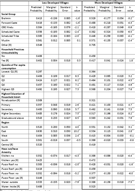
<Table 3>
The PPT of households in the different groups (social, consumption, educational etc.) was
computed through a series of simulations. The first panel of Table 2 show these probabilities for the
LDV and the second panel shows them for the MDV. The PPT against the row panel ‘Social Group”
and the column panel ‘less developed village’ were computed by assuming that all the 19,225
households lived in LDV and were, successively, Brahmin, FC, OBC, SC, ST,
17
developed village’ were computed similarly, but this time assuming that all the 19,225 households
lived in MDV.
The average of these ‘all-Brahmin’ probabilities was 41.3% for the LDV and 52.9% for the
MDV and these are shown in Table 2 against the row labelled ‘Brahmin’. Similarly, the average of the
‘all-Muslim’ probabilities was 56.1% for the LDV and 57.1% for the MDV and these are shown in
Table 2 against the row labelled ‘Muslim’. Since the only factor that was different between these two
calculations – all Brahmin, and all-Muslim - was the households’ religion, with the non-caste
household attributes unchanged, the difference between these PPT (that is, 41.3% and 56.1% for the
LDV and 52.9% and 57.1% for the MDV) could be attributed entirely to differences in religion.30
The marginal probabilities, shown in column 3 of Table 2, represent the differences between
the PPT of the households in the first six social groups and that of (the reference group of) ‘other’
households: so, the marginal probability associated with Brahmins was 41.3-54.9 =13.6 points).
Dividing these marginal probabilities by their standard errors (column 4 of Table 2) yielded the
t-values (column 5 of Table 2); these showed whether these marginal probabilities were significantly
different from zero in the sense that the likelihood of observing these values, under the null hypothesis
of no difference was less than 5% (superscript ** in Table 2) or 10% (superscript * in Table 2). The
results for the LDV show that, except for Muslims, the PPT was significantly lower for every social
group vis-à-vis the reference group of ‘Other’ (comprising Christians, Sikhs, and Jains); there was no
significant difference between the PPT for Muslins (56.1%) and ‘Other’ (54.9%). For the MDV, the
PPT for households in all the groups was significantly lower than that of the reference ‘Other’.
The estimation program also allows one to draw statistical comparisons between the PPT of
different groups. Since some of the discussion about toilets in the home has centred around the
differential behaviour of Hindus and Muslims (Coffey et. al. 2017, p. 64), underpinned by issues of
untouchability, the first port of call in making these comparisons was between Brahmin and Muslim
households: the PPT of Brahmins (41.3%) was significantly lower than that of Muslims (56.1%) in
the LDV but, in the MDV, there was no significant difference between the PPT of Brahmins (52.9%)
30
18
and Muslims (57.1%). A comparison of Brahmin and SC households yielded the opposite results:
now there was no significant difference between the PPT of Brahmin (41.3%) and SC households
(35.6%) in the LDV but, in the MDV, the PPT of Brahmins (52.9%) was significantly higher than that
of the SC (38.2%).
A direct test of the effects of households practicing untouchability on their likelihood of
having a toilet in the house, using the ‘untouchability’ variable (“does anyone in your household
practice untouchability”: yes/no) did not show any significant difference in the LDV between the PPT
of households not practicing (40.6%) and not practicing (40.2%); however, in the MDV, the PPT of
households not practicing untouchability (45.8%) was significantly higher, but only at the 10% level,
than that of households practicing untouchability (41.7%).
These effects, however, were swamped by the effect of other variables. Computing the PPT
by quintile of per capita consumption showed that, in both the LDV and the MDV, the PPT rose
steadily and significantly as one progressed through the quintiles: the PPT, in the MDV, for
households in the highest quintile (56.8%) was significantly higher than that of households in the
fourth quintile (48.1%) while, in both the LDV and the MDV, the PPT for households in the lowest
quintile (29.7% and 36.4%, respectively) was significantly lower than that of households in the next
quintile (40.6% and 42.9%).
A similar story emerges with respect to education, as measured by the highest level of
education of a household adult: the PPT by level of education, in both the LDV and the MDV, rose
steadily and significantly as one progressed through the different education levels: the PPT, in both
the LDV and MDV, for households with a graduate (54.3% and 56.3%, respectively) was
significantly higher than that of households in which the highest level of education was higher
secondary (48.5% and 51.7%, respectively); similarly, in both the LDV and MDV, the PPT for
households with no education (30.9% and 32.1%, respectively) was significantly higher than that of
households in which the highest level of education was primary school (35.7% and 42.1%,
respectively).
Lastly, having an ancillary amenity – whether a separate kitchen or a pucca floor or roof or a
19
amenity compared to not having that amenity: for example, in both the LDV and the MDV, the PPT
for households with a separate kitchen (42.5% and 47.2%) was significantly higher than that for
households without a separate kitchen (35.2% and 38.6%); in both the LDV and the MDV, the PPT
for households with an inside’ water supply (48.8% and 52.3%) was significantly higher than that for
households in which the water supply was outside (33.3% and 38.6%).
6. Post-defecation Handwashing
The IHDS-2011 gave information on the post-defecation handwashing habits of households
both in terms of whether household members washed their hands (never, sometimes, usually, always)
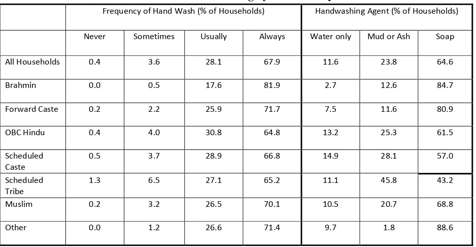
and in terms of what they washed their hands with (water only, mud or ash, soap). Table 4 shows the
percentage of households by social group in terms of the frequency and the method of their hand
washing habits.31
<Table 4>
Table 4 shows that 67.9% of households washed always washed their hands: Brahmins were
the most frequent hand washers (81.9% of persons in Brahmin households always washed their hands)
and persons in OBC, SC, and ST households were the least frequent (64.8% of those in OBC
households, 66.8% of those in SC households, and 65.2% of those in ST households always washed
their hands after defecating). In terms of the method of hand wash, 84.7% of persons in Brahmin
households used soap compared to only 61.5% in OBC households, 57% in SC households, and
45.8% in ST households.
Since the social groups differed in other attributes like education, incomes, water supply,
household amenities, isolating the handwashing habits of the social groups requires one to control for
these non-caste/religion variables. The first step in doing so was to construct a variable hi which
assumed values over rural households, indexed i, such that hi =1 if members of the household usually
oralways washed their hands with soap after defecating and hi =0, otherwise.
32
The IHDS-2011
showed, after grossing up using the survey’s sample weights for households, that the variable hi took
the value 1 (usually/always washed with soap) for 85% of Brahmin households, 80.8% of FC
31
The numbers in Table 4 have been grossed up using the IHDS-1011 household weights, FWT. 32
20
households, 60.8% of OBC households, 56.5% of SC households, 42.5% of ST households, 68.3% of
Muslim households, and 88.4% of ‘other’ households.
Following the methodology detailed in sections 3 and 4 of this paper, a logit model was
estimated with hi as the dependent variable and with the following as determining variables: (i) social
group (subsection A); (ii) Income and Education (subsection B); (iii) Region (subsection C); (iv)
Other Housing Amenities: toilet, kitchen; pucca roof and floor; water supply inside dwelling or
compound (subsection D); (v) whether (some members of) the household practiced untouchability
(subsection E); (v) village type: less or more developed village.
<Table 5>
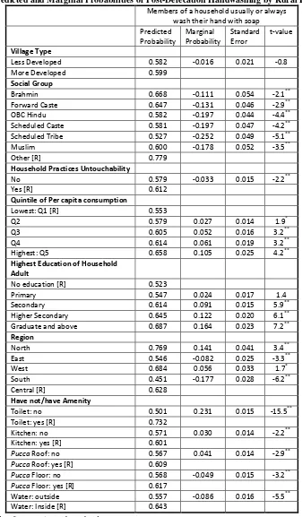
The predicted probability of a household’s members (usually or always) washing their hands
with soap (hereafter, abbreviated to predicted probability of hygiene or PPH) was computed
separately, with respect to every determining variable noted above. The PPH of households in the
two different village types – less and more developed – were computed by first applying the less
developed village coefficient to all the 18,836 households in the estimation sample and computing the
average likelihood of households having a toilet under this ‘all-LDV’ scenario and then, applying the
more developed village coefficient to all the 18,836 households in the estimation sample and
computing the average likelihood of households having a toilet under this ‘all-MDV’ scenario. As the
first item of Table 5 shows, the PPH was not significantly different between the two village types
(58.2% and 59.9% for, respectively the LDV and the MDV) and hence the interaction between village
type and the other variables, which underpinned the econometric work of section 4, is not pursued
here.
The PPH of households in the different groups (social, consumption, educational etc.) were,
as with the PPT of sections 3 and 4, computed through a series of simulations. The PPH against the
row labelled ‘Brahmin’ were computed by assuming that all the 18,836 households in the estimation
sample were Brahmin and computing the average likelihood of households practicing ‘hygiene’ (the
PPH) under this ‘all-Brahmin’ scenario.33 The average of these ‘all-Brahmin’ probabilities was
33
21
66.8%; this is shown in Table 5 against the row labelled ‘Brahmin’. Similarly, the PPH of Muslims
was 60% using the same methodology.
This difference between Brahmins and Muslims in their predicted probability of hygiene was
not significantly different from zero; nor was there a significant difference between the PPH for
Muslims the OBC. On the other hand, the PPH was significantly higher for Brahmin households than
for OBC, SC, and ST households. The results from Table 5 show that, the PPH for households in all
the groups was significantly lower than the 77.9% PPH for the ‘other’ group.
The predicted probability of hygiene was significantly higher for households in which
someone practiced untouchability (61.2%) compared to households in which no one practiced
untouchability (57.9%). This suggests that the former type of households were concerned not just with
ritual purity but also with actual cleanliness!
The PPH of households rose with the quintile of consumption in which they were placed –
from a low of 55.3% for households in the lowest quintile to a high of 65.8% for households in the
highest quintile. Similarly, the PPH of households rose with the highest education level of an adult in
the household: households in which adults did not have any education had a PPH of 55.3% compared
to a PPH of 61.4% for households with at least one adult educated to secondary level, 64.5% for
households with at least one adult educated to higher secondary level; and 65.8% for households with
at least one adult who was a graduate.
The PPH of households also depended upon the amenities within their dwellings. Most
particularly, households having a toilet had a significantly higher PPH than households which did not
have a toilet (73.2% versus 50.1%). For a variety of plausible reasons – for example, difficulty of
carrying soap and sufficient water to wash one’s hands ‘on site’ or forgetting to do so on one’s return
home – defecating in the open also meant compromising on personal hygiene. Households that had a
water supply within the dwelling or its compound were significantly more like to practice hygiene
(PPH of 64.3%) than households whose water supply was outside the dwelling’s compound (PPH of
55.7%).
22
This paper put forward a hypothesis to argue à la Duesenberry (1967) that the social context
in which households were placed was an important factor in deciding whether to have a toilet within
their dwelling. This hypothesis was tested by comparing the demand for toilets in “less developed” to
that in “more developed villages”. The instrument for making this comparison was an econometric
model which allowed every household variable (income, education, non-toilet dwelling amenities
etc.), which might impact upon this demand, to be influenced by the type of village in which the
household resided. The results, detailed in Table 2, showed that ceteris paribus households were
significantly more likely to have a toilet in more developed (44.7%) than in less developed villages
(40.7%). This finding persisted at a more disaggregated level: households in the lowest and highest
quintiles of consumption, households in which the highest adult education level was primary or
secondary, households in most of the regions, were all ceteris paribus households significantly more
likely to have a toilet in more developed, rather than less developed, villages. Equally importantly,
households which had an existing amenity (separate kitchen, pucca roof or floor, inside water supply)
were more likely to also have a toilet if they lived in more developed, compared to less developed,
villages.
Given that some of the current literature on sanitation in India denigrates the process of
development as an instrument of change in defecation habits (from outdoor to indoor) and
emphasises, instead, the role of caste and untouchability in inhibiting change – and, indeed, even
engendering a preference for open defecation among high-caste Hindus – the importance of this result
cannot be overemphasised. For example, Coffey et. al. (2014) write about a “revealed” preference for
open defecation, allied to distaste for having a toilet within the home, by (Hindu) Indians. The
combined effect of preference and distaste then renders futile any governmental toilet-building
program: toilets may be built but they will not be used.
The results reported in this paper show, however, that the link between the practice of
untouchability and the demand for toilets is more nuanced than that articulated, for example, by
Spears and Thorat (2015) in a paper based on IHDS-2011 data and using responses to the same
untouchability question used in this paper. It is true that the raw data shows a greater proportion of
23
which someone practiced untouchability (43%). Nevertheless, to conclude from this that there was a
robust and significant association between households practising untouchability and the presence of
toilets in their homes - and, indeed, that this association was primus inter pares among other possible
associations – is, as this paper shows, simply wrong.
After controlling for other variables, allowing the effects of variables to vary between
village-types (less and more developed), and employing the methodology of “recycled predictions”
(described earlier), this paper shows that, based on whether or not they practiced untouchability, there
was no difference between households in less developed villages in their predicted probabilities of
having a toilet. In more developed villages, however, households practicing untouchability were
significantly less likely at the 10%, but not at the 5%, level to have a toilet compared to households
that did not practice untouchability (Table 3: 41.7% versus 45.8%). More to the point, as shown
earlier, the size of the untouchability effect on the likelihood of households having a toilet was
swamped by the effects of other variables: education, consumption, and ancillary facilities.34
Over and above the answers to the untouchability question in IHDS-2011, there could, of
course, also be shards of ritual pollution and untouchability in say, the behaviour of Brahmins
vis-à-vis Muslims regarding the presence of toilets in the home. According to Coffey et. al. (2017, p. 64),
“if ideas about pollution and untouchability that have their origins in the Hindu caste system
importantly influence defecation behaviour in rural India, we might expect to find differences in
latrine ownership between Hindus and Muslims.” The results of this paper show that, for less
developed villages, the predicted likelihood of households a having a toilet was, indeed, lower for
Brahmins than for Muslims but, in the more developed villages, there was no significant difference
between the two groups in this predicted probability. Moreover, the likelihood of Brahmin
households having toilets was significantly higher in the more developed, compared to the less
developed, villages while, for Muslim households it was unchanged between the two village types.
34
24
This leads again to the central hypothesis of this paper. Whatever inhibitions Brahmins may
have about having a toilet in the home – where these inhibitions may, in part, be derived from
considerations of ritual pollution – were restricted to Brahmin households in less developed villages.
The developmental process involved in moving from less developed to more developed villages swept
away these inhibitions until, in the latter type of village, Brahmins were as likely to have toilets as
Muslims.
Separate from the spread of germs through open defecation is also the spread of germs
through lack of personal hygiene, specifically through not washing one’s hands with soap after
defecating. Now the predicted likelihood of Brahmins being “hygienic” was at 66.8% higher than
the Muslim 60%. This would suggest that some or all of the cons of open defecation of Brahmin
vis-à-vis Muslims was clawed back by the pros of greater personal hygiene. Moreover, the practice of
untouchability actually promoted hygiene, with members of households in which someone practiced
untouchability being more likely to habitually wash with soap than members of households in which
no one practiced untouchability.
This leads to the policies that the Indian government should pursue in order to reduce, if not
eliminate, open defecation. First, the government’s toilet building program seems to be working both
in terms of the proportion of the rural households having toilets and in terms of the usage of existing
toilets. A 2017 Survey covering 140,000 households found that the number of rural households
without a toilet has fallen from over a half (as per the 2011 Census) to under one-third. Moreover,
toilets in nine out of ten households which had a toilet were actually using them (Zainulbhai, 2017).
In addition to building toilets, which incidentally are all of the pit latrine type, the government needs
to either subsidise, or provide them with cheap credit in the form of ‘toilet loans’, households which
are prevented from installing flush toilets because their high cost. Lastly, the government needs to
improve sewage and water supply in villages since these facilities complement toilet installation and
use. But, above all, one needs to avoid the nihilism implicit in the idea that the problem of open
defecation in India is an intractable one because caste, ritual pollution, and untouchability instil in
26
Table1: Housing Amenities by Location and Social Group of Household§
Percentage of Households with Amenity Toilet in House Separate
Kitchen
Water Supply in House or Compound
Pucca Roof* Pucca Floor**
All Households 52.6 54.9 50.6 64.3 59.3
Location of Households
Metropolitan Urban 96.6 74.5 76.9 87.3 97.4 Other Urban 83.5 71.7 70.2 78.5 89.7 More Developed Villages 45.2 53.6 46.9 59.6 60.0 Less Developed Villages 31.1 42.0 36.6 54.7 33.2
Social Group (Rural Households)
Brahmin 50.6 60.9 48.9 72.4 54.5 Forward Caste 54.1 59.5 50.7 64.9 61.8 OBC Hindu 32.9 45.5 40.7 57.8 48.5 Scheduled Caste 27.2 39.9 34.9 56.1 49.2 Scheduled Tribe 26.5 42.1 25.6 36.9 22.3 Muslim 51.7 45.4 51.6 55.3 37.5 Other*** 91.6 87.0 76.1 76.3 90.0
§
Figures areobtained after grossing up using sample weights for households
*
Asbestos, Metal, Brick, Stone, Concrete. ** Not mud or wood. *** Christian, Sikh, Jain
27
Figure 1: Percentage of Rural Households Without a Toilet And Other Amenities
Source: Own calculations from IHDS-2011
66.3
51.1
68.3
0 10 20 30 40 50 60 70 80
Do No Have Toilet And Other Amenity
Separate Kitchen
Pucca Roof
28
Figure 2: Percentage of Rural Households With A Toilet But Without Other Amenities
Source: Own calculations from IHDS-2011
30.5
29.8
33.3
28 29 30 31 32 33 34
Do Not Have Amenity But Have a Toilet
Separate Kitchen
Pucca Roof
29
Table 2: Differences between Village Types in the Predicted Probabilities of Rural Households Having a Toilet§
Predicted Probability in Less Developed Villages Predicted Probability in More Developed Villages Difference in Predicted Probabilities Standard Error of Difference t-value
All Households 0.405 0.447 -0.042 0.017 -2.4** Brahmin 0.413 0.529 -0.115 0.049 -2.3** Forward Caste 0.416 0.488 -0.072 0.033 -2.2** OBC Hindu 0.384 0.418 -0.034 0.023 -1.5 Scheduled Caste 0.356 0.382 -0.026 0.031 -0.8 Scheduled Tribe 0.385 0.446 -0.062 0.048 -1.3 Muslim 0.561 0.571 -0.010 0.045 -0.2 Other 0.549 0.705 -0.156 0.092 -1.7 No Untouchability 0.406 0.458 0.052 0.020 -2.6** Yes Untouchability 0.402 0.417 0.015 0.026 -0.6 Q1 of per-capita
consumption
0.297 0.364 -0.067 0.025 -2.6**
Q2 of per-capita consumption
0.406 0.429 -0.022 0.025 -0.9
Q3 of per-capita consumption
0.424 0.464 -0.040 0.026 -1.6
Q4 of per-capita consumption
0.457 0.481 -0.024 0.027 -0.9
Q5 of per-capita consumption
0.492 0.568 -0.076 0.031 -2.4
No education 0.309 0.321 -0.011 0.025 -0.5 Primary 0.357 0.421 -0.064 0.027 -2.4** Secondary 0.400 0.462 -0.062 0.021 -2.9** Higher Secondary 0.485 0.517 -0.032 0.029 -1.1 Graduate and
above
0.543 0.563 -0.020 0.037 -0.5
North 0.520 0.551 -0.031 0.060 -0.5 East 0.630 0.534 0.096 0.044 2.2** West 0.404 0.415 -0.011 0.038 -0.3 South 0.301 0.399 -0.098 0.039 -2.5** Central 0.320 0.419 -0.099 0.027 -3.6** Kitchen: no 0.352 0.386 -0.034 0.026 -1.3 Kitchen: yes 0.425 0.472 -0.047 0.019 -2.4**
Pucca Roof: no 0.383 0.428 -0.045 0.025 -1.8*
Pucca Roof: yes 0.419 0.459 -0.040 0.019 -2.1**
Pucca Floor: no 0.352 0.377 -0.025 0.023 -1.1
Pucca Floor: yes 0.446 0.507 -0.061 0.023 -2.7**
Water: outside 0.333 0.488 -0.155 0.020 -7.9** Water: Inside 0.386 0.523 -0.138 0.018 -7.5**
§
Estimated on data for 19,225 rural households
**
Significant at 5%; * significant at 10%.
See Notes to Table 1
30
Table 3: Predicted and Marginal Probabilities of Rural Household Having Toilets by Type of Village§
Less Developed Villages More Developed Villages
Predicted Probability Marginal Probability Standard Error t-value Predicted Probability Marginal Probability Standard Error t-value Social Group
Brahmin 0.413 -0.136 0.085 -1.6* 0.529 -0.177 0.054 -3.2** Forward Caste 0.416 -0.133 0.082 -1.6* 0.488 -0.218 0.051 -4.3** OBC Hindu 0.384 -0.165 0.079 -2.1** 0.418 -0.287 0.049 -5.9** Scheduled Caste 0.356 -0.193 0.082 -2.4** 0.382 -0.324 0.050 -6.5** Scheduled Tribe 0.385 -0.164 0.083 -2.0** 0.446 -0.259 0.063 -4.1** Muslim 0.561 0.012 0.085 0.1 0.571 -0.135 0.057 -2.4**
Other [R] 0.549 0.705
Household Practices Untouchability
No 0.406 0.458
Yes [R] 0.402 0.004 0.018 0.3 0.417 0.041 0.024 1.8*
Quintile of Per capita consumption
Lowest: Q1 [R] 0.297 0.364
Q2 0.406 0.109 0.017 6.3** 0.429 0.065 0.020 3.2** Q3 0.424 0.127 0.021 6.1** 0.464 0.101 0.022 4.5** Q4 0.457 0.160 0.022 7.1** 0.481 0.117 0.024 4.9** Highest: Q5 0.492 0.195 0.027 7.3** 0.568 0.204 0.027 7.6**
Highest Education of Household Adult
No education [R] 0.309 0.321
Primary 0.357 0.048 0.019 2.6** 0.421 0.100 0.021 4.7** Secondary 0.400 0.090 0.016 5.7** 0.462 0.141 0.019 7.5** Higher Secondary 0.485 0.176 0.024 7.5** 0.517 0.196 0.024 8.2** Graduate and above 0.543 0.233 0.027 8.5** 0.563 0.242 0.031 7.9**
Region
North 0.520 0.200 0.050 4.0** 0.551 0.132 0.042 3.1** East 0.630 0.310 0.030 10.2** 0.534 0.115 0.041 2.8** West 0.404 0.085 0.036 2.4** 0.415 -0.004 0.033 -0.1 South 0.301 -0.019 0.037 -0.5 0.399 -0.020 0.033 -0.6
Central [R] 0.320 0.419
Have not/have Amenity
Kitchen: no 0.352 -0.074 0.017 -4.3** 0.386 -0.086 0.020 -4.4** Kitchen: yes [R] 0.425 0.472
Pucca Roof: no 0.383 -0.036 0.018 -2.0** 0.428 -0.031 0.020 -1.6*
Pucca Roof: yes [R] 0.419 0.459
Pucca Floor: no 0.352 -0.094 0.018 -5.2** 0.377 -0.130 0.022 -6.0*
Pucca Floor: yes [R] 0.446 0.507
Water: outside 0.333 -0.155 0.020 -7.9** 0.386 -0.138 0.018 -7.5** Water: Inside [R] 0.488 0.523
§
Estimated on data for 19,225 rural households
**
Significant at 5%; * significant at 10%; [R] denotes reference category
See Notes to Table 1
31
Table 4: Post-Defecation Handwashing by Social Group of Household
Frequency of Hand Wash (% of Households) Handwashing Agent (% of Households)
Never Sometimes Usually Always Water only Mud or Ash Soap
All Households 0.4 3.6 28.1 67.9 11.6 23.8 64.6
Brahmin 0.0 0.5 17.6 81.9 2.7 12.6 84.7
Forward Caste 0.2 2.2 25.9 71.7 7.5 11.6 80.9
OBC Hindu 0.4 4.0 30.8 64.8 13.2 25.3 61.5
Scheduled Caste
0.5 3.7 28.9 66.8 14.9 28.1 57.0
Scheduled Tribe
1.3 6.5 27.1 65.2 11.1 45.8 43.2
Muslim 0.2 3.2 26.5 70.1 10.5 20.7 68.8
Other 0.0 1.2 26.6 71.4 9.7 1.8 88.6
32
Table 5: Predicted and Marginal Probabilities of Post-Defecation Handwashing by Rural Households§
Members of a household usually or always wash their hand with soap Predicted Probability Marginal Probability Standard Error t-value Village Type
Less Developed 0.582 -0.016 0.021 -0.8 More Developed 0.599
Social Group
Brahmin 0.668 -0.111 0.054 -2.1** Forward Caste 0.647 -0.131 0.046 -2.9** OBC Hindu 0.582 -0.197 0.044 -4.4** Scheduled Caste 0.581 -0.197 0.047 -4.2** Scheduled Tribe 0.527 -0.252 0.049 -5.1** Muslim 0.600 -0.178 0.052 -3.5** Other [R] 0.779
Household Practices Untouchability
No 0.579 -0.033 0.015 -2.2** Yes [R] 0.612
Quintile of Per capita consumption
Lowest: Q1 [R] 0.553
Q2 0.579 0.027 0.014 1.9* Q3 0.605 0.052 0.016 3.2** Q4 0.614 0.061 0.019 3.2** Highest: Q5 0.658 0.105 0.025 4.2**
Highest Education of Household Adult
No education [R] 0.523
Primary 0.547 0.024 0.017 1.4 Secondary 0.614 0.091 0.015 5.9** Higher Secondary 0.645 0.122 0.020 6.1** Graduate and above 0.687 0.164 0.023 7.2**
Region
North 0.769 0.141 0.041 3.4** East 0.546 -0.082 0.025 -3.3** West 0.684 0.056 0.033 1.7* South 0.451 -0.177 0.028 -6.2** Central [R] 0.628
Have not/have Amenity
Toilet: no 0.501 0.231 0.015 -15.5** Toilet: yes [R] 0.732
Kitchen: no 0.571 0.030 0.014 -2.2** Kitchen: yes [R] 0.601
Pucca Roof: no 0.567 0.041 0.014 -2.9**
Pucca Roof: yes [R] 0.609
Pucca Floor: no 0.568 -0.049 0.015 -3.2**
Pucca Floor: yes [R] 0.617
Water: outside 0.557 -0.086 0.016 -5.5** Water: Inside [R] 0.643
§
Estimated on data for 18,836 rural households.
**
Significant at 5%; * significant at 10%; [R] denotes reference category
See Notes to Table 1