An overview of the elementary statistics of correlation, R squared, cosine, sine, and regression through the origin, with application to votes and seats for Parliament

(1)

An overview of the elementary statistics

of correlation, R-squared, cosine, sine,

and regression through the origin, with

application to votes and seats for

Parliament

Colignatus, Thomas

Thomas Cool Consultancy Econometrics

20 April 2018

Online at

https://mpra.ub.uni-muenchen.de/86307/

(2)

An overview of the elementary statistics of

correlation,

R

_{-Squared, cosine, sine, and}

regression through the origin, with application

to votes and seats for parliament

Thomas Colignatus

Econometrician (Groningen 1982) and teacher of mathematics (Leiden 2008)

Abstract

The correlation between two vectors is the cosine of the angle between the centered data. While the cosine is a measure of association, the lit-erature has spent little attention to the use of the sine as a measure of distance. A key application of the sine is a new “sine-diagonal inequality / disproportionality” (SDID) measure for votes and their assigned seats for parties for Parliament. This application has nonnegative data and uses regression through the origin (RTO) with non-centered data. Text-books are advised to discuss this case because the geometry will improve the understanding of both regression and the distinction between descrip-tive statistics and statistical decision theory. Regression may better be introduced and explained by looking at the angles relevant for a vector and its estimate rather than looking at the Euclidean distance and the sum of squared errors. The paper provides an overview of the issues involved. A new relation between the sine and the Euclidean distance is derived. The application to votes and seats shows that a majority of the electorate in the USA and UK, that have District Representation (DR) and not Equal or Proportional Representation (EPR), still tends to have “taxation without representation”.

(3)

D710 Social Choice; Clubs; Committees; Associations,

D720 Political Processes: Rent-seeking, Lobbying, Elections, Legislatures, Voting Behavior D630 Equity, Justice, Inequality, and Other Normative Criteria and Measurement

MSC2010

62J20 Statistics. Diagnostics 00A69 General applied mathematics

28A75 Measure and integration. Length, area, volume, other geometric measure theory 97M70 Mathematics education. Behavioral and social sciences

©Thomas Cool, Scheveningen, CC BY-NC-ND 4.0

1 Introduction

1.1 The subject of discussion

Karl Pearson (1857-1936) designed correlation between two vectors with the de-liberate focus on centered data, namely to capture as much variation as possible. This arrangement also applied to the coefficient of determination,R2 _or _R-squared, between a vector and its estimate.

We now have reason to look at the original and non-centered data, and in particular at nonnegative data. This application arises for votes and the assigned seats for parties for Parliament. When we want equal proportions of votes and seats, or to maximise the association, or to minimise the inequality / disproportionality (ID), then it would not make sense to center the data. Having a vector of seat shares at a constant distance of a vector of vote shares would be rather curious. For such non-centered data we apply regression through the origin (RTO), see Kozak and Kozak(1995) andEisenhauer (2003). Textbooks tend to warn against dropping the constant in the regression, since it is better to test whether modeling errors show up in an estimated constant, yet in this case RTO appears to be the proper approach.

Obviously, both Pearson’s centered data and RTO share the property that the con-stant is zero, yet remarkably there are some (conceptual) differences for nonnegative data. This article will use this framework of nonnegative vectors, following Coligna-tus(2017c),Colignatus(2017d),Colignatus(2018a),Colignatus(2018b),Colignatus (2018c), but potentially some properties might be generalised for other data.

Pearson also concentrated on the cosine as a measure of similarity. The literature has spent little attention to the use of the sine as a measure of distance. For shares of votes and seats one might say that they are 97% close but the literature on votes and seats has focussed on developing measures of inequality / disproportionality, as people might be more sensitive to the 3% dissimilarity. Colignatus(2018b), discusses measures for votes and seats, and develops the new sine-diagonal inequality / dis-proportionality (SDID) measure. SDID uses not only the sine but also the square root on the sine, as a magnifying glass for small values, like the logarithm in the Richter scale. Colignatus(2018a) gives a more general perspective on distance and norm, and rejects the Aitchison geometry for compositional data for this comparison of votes and seats. 1

There are particular aspects in voting, like majority switches, that are not relevant for other applications. The sine measure is more sensitive than the angular distance, and also interesting since it links up to regression, since R2 finds its translation in RTO as the squared cosine of the angle between the vectors. A new finding in Section 4.8 below is a direct relation between the sine and the Euclidean distance between two vectors.

Our objective here is to provide an overview of the elementary statistics of

cor-1

Comparing votes and seats is a topic of itself, and it is another topic for example to explain votes by say the economy. In the latter, the log or logit transformations could still be used, though

(5)

relation, R-squared, cosine, sine, and regression through the origin (RTO), with application to votes and seats for Parliament. While our focus is on the relevance for statistics -Mood and Graybill(1963) p1 describe statistics as “the technology of the scientific method” - and while we will have an eye on education in statistics, we cannot avoid highlighting aspects of votes and seats, since this content determines the analysis. For earthquakes there exists the Richter scale, but for votes and seats there isn’t yet a similar “change” measure, while the advice now is to use SDID.

We will look at the same issue from different perspectives - statistics versus the issue of content on electoral systems, correlation versus trigonometry, theory versus education - and thus cannot avoid repetition, which however helps to identify that we are speaking about the same issue.

We use x for a real vector, _kx_k = √x′_x _{for the norm of} _{x, and} _k_y₋_x_k _{for the} Euclidean distance betweenx andy. Normalised are x∗ ₌_x/_k_x_k _and _y∗ ₌_y/_k_y_k_. There is alsoθ for the angle betweenxandy. Linear algebra provides an expression for the cosine of this angle, as Cos[x, y] =x′_y/√_x′_{x y}′_y₌_x∗ ′_y∗_{, i.e. the improduct} of the normalised vectors on the unit circle. Cos is essentially the projection divided by the radius 1, see also the discussion and graph below. 2

Thenθ= ArcCos[Cos[x, y]]. The formula for the cosine is scale invariant, as the angle does not change for positive scalarsλandµ, with Cos[x, y] = Cos[λ x,µ y].

1.2 Votes and seats

Letvbe a vector of votes for parties andsa vector of their seats gained in the House of Commons or the House of Representatives. We discard zeros invand use a single zero insfor the lumped category of “Other”, of the wasted vote, for parties that got votes but no seats. Let V =1′_v _{be total turnout and} _S ₌ ₁′_s _{the total number of} seats, andw =v/V andz =s/S the perunages. For presentation we will use 10w and 10zand the range [0, 10] in general. For votes and seats, percentages [0, 100] generate too much an illusion of precision, while [0, 1] generates too many leading zeros. Distance measures on [0, 10] read as an inverted (Bart Simpson) report card (with much appreciation for a low score). 3

In political science, the main current inequality / disproportionality (ID) measures are, conventionally for percentages but now with 10: 4

2

For projection ofyontox, the projection matrixP =x x′_/x′_x_{, so that}_{P y}₌_{x x}′_y/x′_x₌_{b x}_.

Normalisingxandyonto the unit circle shows the relation to Cos, see below.

3

Ð(unicode 00D0,M athematicaEsc D- Esc, Word: ctrl ’ + Shift D) can be used as the formal symbol of base 10. The official name of the letter is Capital Eth, but for_Ð= 10 the pronunciation “deka” is more appropriate. With universal constantH = -1 “eta”, then_ÐH _{would be “decim”}

= “per 10”. Thus 10% = 1_ÐH_{= 1 decim. We would state “5.4 per 10” as 5.4 decim, 5.4 /}_Ð

or 5.4_ÐH_{, or 0.54. On}_H _{= -1 see}_{http://community.wolfram.com/groups/-/m/t/1313302}_.

4

We might leave out the factor 10 in these definitions, and use 10 only for presentation, but for SDID the factor 10 is a key design feature, and thus the others are best at the same scale. Other presentations introduced the scale via the inputs, like 10w and 10z, but it is better to keepw

(6)

• Absolute difference / Loosemore-Hanby (ALHID): 10 Sum[Abs[z-w] / 2]. The division by 2 corrects for double counting. An outcome of 1 means that one seat in a House of 10 seats is relocated from equality / proportionality.

• Euclid / Gallagher (EGID): 10 p

Sum[ (z₋w)2_{/ 2] = 10}_||_z₋_w_||_/√₂_{, with} the first form for comparisons. For two parties this equals ALHID.

• χ2 _{/ Webster / Sainte-Laguë (CWSID): 10 Sum[w}₍_z/w₋₁₎2_{] = 10 Sum[}₍_z₋ w)2_{/w]. The Chi-Square expression has nonzero}_{w. One can compare CWSID} with ALHID = 10 Sum[wAbs[z/w- 1] / 2] and EGID = 10p

Sum[w2₍_z/w₋₁₎2_{/ 2]}

• The difference in shares for the “largest” party, i.e. with the most seats: 10 (zL - wL). This is an easy, rough and ready indicator with some history in the literature, and Shugart and Taagepera (2017) p143 show remarkably that EGID _≈10 (zL -wL).

The proposed newsine-diagonal inequality / disproportionality(SDID) measure has the formula SDID[v, s] = sign 10p

Sin[v, s]. The sine is invariant to scale: Sin[v, s] = Sin[w, z]. Withk= Cos[v,s] given by linear algebra, we might useθ= ArcCos[k] and then find Sin[v, s] = Sin[θ] but we can also use Sin[θ] = √1₋k2 _directly. The additional square root on Sin works as a magnifying glass for inequalities / disproportionalities. The sign indicates majority switches, and is 1 for zero or positive covariance and -1 for negative covariance. 5

ALHID and EGID have a division by 2 to remain in the [0, 10] range, while Sin achieves the same purpose without such division. The newly derived relation inSection 4.8 explains this.

To clarify the distinction between the new proposal and the conventional mea-sures in political science, Figure 1 gives ALHID (blue) and SDID (red), and the intermediate steps given by the angle (yellow) and sine itself (green). 6

For two parties normalised to [0, 10] we plot withseats= _{t, 10 -t_}, witht the seats for the first party. We also consider opposite valuesvotes =_{10 -t, t_} = 10 -seats. Since this implies negative correlation, the SDID becomes negative, but the plot gives the absolute value. To wit:

• The angular measure (AID) is 10θ/90◦₍_yellow_{). Since we look at nonnegative} vectors, the maximum angle is 90◦_.

• The sine plotted is 10 Sin[θ] (green). For small angles Sin[θ] _≈ θ (slope 1) especially in radians. There is a large difference between Sin[θ] andθ/90◦_.

The key point of Figure 1is that the SDID indeed works like a magnifying glass to determine inequalities / disproportionalities in votes and seats. This relates to the Weber-Fechner law on psychological sensitivity. 7

5

In speech, with the similarity of “sine” and “sign”: then use “sinus” and “signum”.

6

(7)

When a frog is put into a pan with water at room temperature and subsequently is slowly boiled it will not jump out. When a frog is put into a pan with hot water it will jump out immediately. People may notice big differences between vote shares and seat shares, but they may be less sensitive to small differences, while these differences actually can still be quite relevant for the decision to jump out. For this reason, the SDID uses a sensitivity transform. Like with the Richter scale, it will now be easier to relate the smaller values to the larger values. At the valuest= 4.5 or 5.5, when the absolute distance ALHID registers a 1 on a scale of 10, SDID generates a staggering 4.4 on a scale of 10, which outcome better relays the message that this difference is alarming.

2 4 6 8 10

Share seats first party, 2nd party opposite

Votes opposite 2

4 6 8 10

[image:7.595.147.454.270.421.2]

Abs, Angle, Sin, Sqrt[Sin]

Figure 1: Plot ofd[votes, seats] for votes= 10 - seatsandseats=_{t, 10 -t_}, for d= Abs/2, AngularID, Sine, and_|SDID_|(eliminating the latter’s negative sign)

As another example: When votes _{4.9, 5.1_} are translated into seats then the absolute difference (ALHID) and the Euclidean distance (EGID) regard outcomes

{4.8, 5.2_}or_{5.0, 5.0_}as at the same distance, namely 0.1 seat difference (correcting for double counting), while common sense and the sine would hold that the seats

{4.8, 5.2_} are closer to the votes and less disruptive than the seats _{5.0, 5.0_} that suggests that there is equality. The values are: 10 Sin[_{4.9, 5.1_},_{4.8, 5.2_}] = 0.1998 < 0.19996 = 10 Sin[_{4.9, 5.1_}, _{5.0, 5.0_}]. 8

These values are so close together, though, that also the magnifying glass SDID hardly sees a difference: 1.41351 < 1.41407. However, the latter values are still at the high level or 1.4 on a scale of 10, rather than at the low value of 0.1 on a scale of 10 for ALHID.9

7

Wikipedia is a portal and no source:

https://en.wikipedia.org/wiki/Weber%E2%80%93Fechner_law

8

We didn’t divide the sine by 2 to correct for double counting. If we would do so then 0.1998 / 2

≈0.1 or the ALHID score. But then we would have to multiply by 20 instead of 10 to get to the [0, 10] range again. For small values Sin[w, z] = Sin[θ]≈θ ≈ kz/kzk −w/kwkk. For the unit simplex we might considerkz−wk/pkzk kwkusing the geometric mean.

9

(8)

Table 1 contains the real world example of the US House of Representatives of 2016 (435 seats) and the UK House of Commons 2017 (650 seats). SDID properly conveys the insight that there is shocking inequality / disproportionality.

Table 1: Votes and seats in the USA 2016 and UK 2017 10

USA, House, 2016,S = 435 UK, House, 2017,S = 650

Party Votes Seats Party Votes Seats

Republicans 4.91 5.54 Conservatives 4.22 4.88

Democrats 4.80 4.46 Labour 3.99 4.03

Other 0.29 0 Other 1.79 1.09

100% 10 10 100% 10 10

10 (z_L -w_L) 0.63 10 (z_L -w_L) 0.66

ALHID 0.63 ALHID 0.70

AID 0.67 AID 0.92

SDID 3.2 SDID 3.8

1.3 Structure of the paper

The square root within SDID is psychologically important and only a presentation feature of descriptive statistics. This present discussion collects the key steps in Colignatus(2018b) for the content of statistics and targets at an overview. Part of the present text has already been used on my weblogColignatus (2017c).

The next section provides notation and basics. The subsequent section places our topic within the perspective of the statistical triad of experimental design, description and decision. Subsequently we apply the cosine and sine for nonnegative data, and state the relevant formulas. We close with a summary of the findings.

The reader might peek at Table 2 for the different models, to see what this discussion is about specifically. I have considered putting this table up front, but it is better to rekindle awareness about the basics before delving into the models.

PM 1. See Colignatus (2007) for the approach with determinants rather than angles - as area and volume might generalise easier to more dimensions than the angle, that remains stuck to the 2D plane created by the two vectors. PM 2. There is the notion of “distance correlation”11

but the Pearson correlation remains relevant here precisely because of the linearity contained in the notion of equality / proportionality. PM 3. There is “least angle regression” but this is different. 12

We remain in the realm of “simple regression”. 13

a House of 100 is relocated. The ALHID recovers the 1% but SDID magnifies to a score of 14 on a scale of 100. This 1% of the US House is 4.35 seats, and of the UK House 6.5 seats, or, with double effect 8.7 and 13 seats. This 1% might make quite a difference. The value of 1.4 on a scale of 10 would seem to be acceptable as the indication that something is wrong.

10

The interpretation of this table requiresSection 5.3.

11

Wikipedia is a portal and no scource. https://en.wikipedia.org/wiki/Distance_correlation

12

https://en.wikipedia.org/wiki/Least-angle_regression

13

(9)

2 Notation and basics

2.1 Well-known basics

We underline variables for the centered valuex=x -x. The angle¯ θ is between the centered valuesx andy. The Pearson correlation coefficient is r[x, y] = Cos[x - x,¯ y- y] = Cos[x,¯ y] = Cos[θ], so that θ= ArcCos[r[x, y]]. The covariance ofx andy is the improduct of the centered values, divided by the number of observationsn, or cov[x, y] = x′_{y/n. Using covariance, the correlation coefficient}_{r[x, y] = cov[x, y] /} p

cov[y, y]cov[x, x]. See e.g. Egghe and Leydesdorff(2009) for a visualisation of the shift towards centered data, andTheil(1971) p165 for a discussion of the geometric meaning thatr = Cos[θ].

Along (1) θ and (2) θ, we also consider the linear cases of (3) the “regression through the origin” (RTO) forygivenx,without a constant, and (4) the “regression” in general, with a standard constant, hence fory given x. For linearity, the standard case with a constant may also be formulated in terms ofyandx,but some formulas then require the mention of the means. The symbolyˆdenotes the estimate ofy, but eandˆedenote merely different kinds of error.

For (4) with centeredy = X b+eˆfor matrixX, then y′_y ₌_b′_X′_Xb_{+ ˆ}_e′_e_ˆ_using X′_ˆ_e_{= 0. This is commonly expressed as SST = SSX + SSE. In this,}_y′_y _{= SST =} sum of squares total,ˆe′_ˆ_e_{= SSE = sum of squared errors, and SSX = sum of squares} of the explanation = SST - SSE.14

The coefficient of determination is R2 _{= SSX / SST. Thus} ₁₋ _R2 _{= SSE/} SST. For the calculation of SST and SSE we must use centered data, though the regression itself might also be formulated as y = Xb + ˆe with a column of 1 in X for the constant. With n observations and m explanatory variables in X, the root mean squared error (RMSE) adjusted for the degrees of freedom is RMSE = p

SSE/(n₋m). Colignatus (2006) discusses the sample distribution of (adjusted) R-squared. When the (explanatory) variables are given without measurement errors then there is not a “population” but a “space”, and the relevant parameter forR is best denoted asρ[X]to express the conditionality on the data.

While the coefficient of determination R2 _{in this setup seemingly has an} inde-pendent definition as SSX / SST, it appears that it is actually the square of the correlationr between yand its estimate y. It might be possible to present this iden-ˆ tity as a great insight and wonder, but it is better to infer that such independence of definition actually wasn’t possible. It is better to start withr[y,yˆ]and then show that steps in its calculation can be abbreviated as SST, SSX and SSE. TheR2_{for two} vectors thus is the squared cosine of the angleθ between the centered values. The root mean squared error (RMSE) then relates to Sin[θ] = √1₋R2 ₌p

SSE/SST, namely as RMSE = Sin[θ] p

SST/(n₋m).

The angle itself is a measure of distance. The angle divided by 360◦_{gives a measure}

14

(10)

in [0, 1]. See Colignatus (2015a) - and below - for a suggestion to measure angles on [0, 1] anyway, using the plane itself as the unit of account, and to speak about turns. When it doesn’t matter whether the angle is positive or negative, then 180◦ would be a relevant maximum. For nonnegative data the relevant maximum is 90◦_. Subsequently 1 minus such value is an angular measure of association.

The cosine is a measure of association too. Some have suggested to take 1 - Cos as a distance, calling it “cosine distance”, but this actually is not a metric, seeDongen and Enright(2012). The latter authors clarify that the sine and its root are a metric. Using Sin[θ] =√1₋R2 _{as a measure of distance might be dubious. The square root} causes a management of the signs, and when the angle is larger than 90◦_{, then the} same values of the sine can only be distinguished by looking at the sign of the cosine again. It might well be that this present discussion remains relevant for nonnegative vectors only.

2.2 Regression through the origin (RTO), for nonnegative vectors

At stake now is the use ofθ of the original and non-centered vectors, which leads us to regression through the origin (RTO). Also, we consider nonnegative vectors. In this case, the angle between the vectors is between 0 and 90◦_.

Withk= Cos[θ] = Cos[x, y], and faced with a choice of a distance measure, there is no fundamental difference between usingθ= ArcCos[k] or Sin[θ] =√1₋k2_{. The} advantage of using the sine instead of the angle is that we have some interpretations in terms of regression because of the cosine. Also,θ/90◦ _{has a lower slope than the} sine at small values of the angle, whence the sine is more sensitive, which fits our purposes. While we can add lengths and angles, we cannot add values of the sine though.

There are slopes b and p from the regressions through the origin (RTO) z = bw + e and w= pz + ε. Then k = Cos[v, s] = Cos[w, z] = √b p. The geometric mean slope is a symmetric measure of similarity of the two vectors. Also Sin[v, s] = Sin[w, z] = Sin[θ] =√1₋b pis a metric and a measure of distance or inequality or disproportionality in general.

All this is straightforward but there are some reasons to call attention to it.

• Political scientists have been looking for a sound inequality / disproportionality measure without finding one, i.e. not finding the sine. They have been setting for the less adequate Euclidean distance EGID discussed (not proposed) by Gal-lagher (1991), though with an awareness that it wasn’t perfect, seeTaagepera and Grofman(2003),Karpov(2008) andKoppel and Diskin(2009). Colignatus (2018b) provides an overall evaluation.

(11)

ˆ

s = Ap[S, v]. This means that the influence of S cannot be neglected as perhaps may be done in “pure” compositional data.

• Compositional data generally would use a log transform (with the geometric av-erage as the mean) and drop one equation because of the addition condition. For the present paper, however, we don’t employ statistical decision theory, with regression as one of its applications, but we employ statistical description (without distinction between true coefficient band its estimate). For determi-nation of the angle between the vectors all elements are relevant, though still with the scalar invariance. Seeming “compositional data” like votes and seats contribute to our understanding of RTO that we consider two errors, not only z =b w+e (used by SDID) but also z= w+ ˜e (used by ALHID, EGID and relatively by CWSID).

The inoptimal situation of discussion in these different though related areas might have to do something with that, remarkably, the angular distance and the sine tend not to be in the textbooks. 15

Currently, errors are related to thenormal distribution. From there, the Euclidean distance,_||y₋yˆ_||=_||eˆ_||=√SSE, is a measure of variation and estimator for true variation, whence regression is explained, and proceeds by minimising SSE to find the normal equations and solve for coefficients. Instead it might make more sense to explain that the angle can be used as a distance measure, and minimizing the angle means maximising the association expressed by Cos[y, y].ˆ For regression with a constant this uses Cos[y, c+b x].

However, a binary regression in RTO hasy=b x+eandyˆ=b x, so that Cos[y, y]ˆ = Cos[y, x] because of scale invariance, so that the angle is fixed. We still require another criterion than the angle betweeny andyˆto find the parameterb.

• For RTO, SSE =e′_e_{= (}_y₋_{b x}₎′₍_y₋_{b x}_{) =}_y′_y₋₂_{b y}′_x₊_b2_x′_{x, and setting} the derivative for b to zero gives a minimum for the value b=y′_x/x′_{x. PM.} On occasion b=p

y′_y/x′_x_{Cos[x, y] may be useful.}

• Fromy=b x+ewe can take the improductx′_y₌_{b x}′_x₊_x′_{e, and set}_x′_e_{= 0}_, so thatb=y′_x/x′_{x. This is shorter but requires geometry instead of calculus.}

The latter approach projectsyontoxand imposes perpendicularity betweenxand e, which meansx′_e_{= 0, so that also Cos[x, e] = Cos[x, y}₋_{b x] = 0. The projection} ofyonxis given byb x, withb=x′_y/x′_{x, using projection matrix}_P ₌_{x x}′_/x′_x_and P y=b x. At this value ofbthe length ofeis smallest. Taking the shortest distance is equivalent to minimising _||e_|| but the geometry avoids the calculus. Figure 2, taken from Colignatus (2011) p143, shows the geometry how Effect y is projected onto Cause x, which determines the size of the Explanation b x, so that Effect y follows from addition of perpendicular Cause b x and Error e. On the LHS, Cause and Effect are normalised onto the unit circle, so that the coefficient is Cos orR at

15

(12)

63%. The RHS is not normalised with coefficientb = 0.546. (In this version of the paper, the LHS has been clarified with the arcs at radius 1 and at radius 0.63.)

Thus there is a geometric approach that is at least as intuitive as the minimisa-tion of SSE with reference to the normal distribuminimisa-tion. The conceptual link between perpendicularx andeand minimal SSE need not be intuitive however, and can only be proven exactly (skipping axiomatic geometry) by looking at the normal equation.

Effect

Cause Explained

Explanation Error

Work Consumption

Effect

Cause Explained

Explanation Error

[image:12.595.146.453.227.356.2]

Work Consumption

Figure 2: Projection of Effect_{4, 9_}on Cause _{11, 3_}16

Both approaches generate the same solution, and there is only the difference in presentation, either via the angles between the vectors or the Euclidean norm of the error. Both relate to the assumption of i.i.d. normal errors, but the latter can also be seen as step 2, when one agrees that it is more informative to start with the use of the angle as step 1, rather than derive the angle as a corollary or be actually silent on it.

My suggestion is that the world of statistics develops a greater awareness of the angle and sine as distance metrics in relation toR-squared, at least for applications of RTO for such nonnegative data. For textbooks in statistics, this particular combina-tion might be regarded as a missing link. The geometry would contribute to a better understanding by students of both regression and the distinction between descriptive statistics (no distinction between b and an estimate) and statistical decision theory (a trueband its estimate).

Shalizi(2015) p19 states that “I have never found a situation where it[R2_]_helped at all.” – see alsoFord(2015). This statement is somewhat curious where minimising the sum of squared errors is equivalent to maximising R2_{, so that} _R2 _{is crucial.}

16

The RHS: The projection of Effectyon Causexgenerates the Explanationb x. Addition ofb x

and perpendicular Errore(from Explanation to Effect) generatesyagain. The LHS: Cause and Effect are on the unit circle (radius 1) and the smaller arrows from the origin are on the circle with radius 0.63. Normalisation ofy =b x +e givesy∗₌_b∗_x∗₊_e∗_{, using} _e∗ ₌_e/_k_y_k_{, and}

b∗₌_b_k_x_k_/_k_y_k_{. Obviously}_b∗_{= Cos[}_{y, x}_{]. Thus the Explanation}_b∗_x∗_{on the LHS gives the Cos,}

in this example 63%. For the Explained part of the Effect we usey∗ ′_y∗₌_b∗_x∗ ′_x∗_b∗₊_e∗ ′_e∗_or

(13)

Obviously one should be careful in interpreting the actual outcome of aR2_calculation, e.g. in specification search.

A view from didactics

In education it happens far too often that a textbook starts a new section with “Now something completely different” while it appears that one essentially has the same topic though only from another perspective. Consider for example_{x, y_}=x + i y =r (Cos[ϕ] + i Sin[ϕ]) = Exp[r + i ϕ]. Or, in fact, that above shortest distance can be found by both projection and calculus, creating the field of analytic geometry. Obviously such perspectives exist and each perspective has something to say for it, and obviously it is a result in itself when one can show the equality. But one also feels rather exasperated, discovering that one only learns different languages for the same.

In the same way for correlation. The “explanation” on correlation, that “correlation between two vectors is the cosine of the angle between the centered data”, is only required because the word “correlation” has been introduced without explicit refer-ence to the basic angularity of the notion. Most students, who first are introduced to “covariance” and correlation by a formula that uses covariance, will miss out on the notion that correlation refers to an angle. Even when this is derived it tends to remain a mystery because students have built up mental maps on “correlation” that tend to be quite different from angles.

Perhaps it was a deliberate decision by Karl Pearson to keep trigonometry outside of the realm of statistics, for fear that the subject might appear more dreadful than needed. Instead, it would be better to make trigonometry more acceptable, see “Trig rerigged” in Colignatus (2015a). Let α be the size of the turn, measured on the angular circle with circumference 1. Consider the values of _{X, Y_} on the unit radius circle, such that X2 ₊ _Y2 _{= 1. The upper case variables} _X _and _Y_, as standard co-ordinates on the unit circle, have the same role as the lower case variables x and y as the standard co-ordinates for the plane. We now define the functional relationships: X=Xur[α]and Y =Yur[α]. With each value ofX = Xur there is a Y = Yur on the unit radius circle, and the angle α that gives the size of the turn in [0, 1]. This approach avoids the mysterious names and uninformative labels “sine” and “cosine”, and avoids the needless calculation that 90◦ _{is a quarter} of 360◦_{. Useful is also}_Θ_{= 2π, pronounced as “archi” from Archimede, and written} with capital theta. 17

Obviously Xur[α] = Cos[αΘ] and Yur[α] = Sin[αΘ] in radians. The only reason to keep using sine and cosine defined on the unit radius circle itself is that their derivatives in radians translate into each other. Once students have learned trigonometry with Xur and Yur while avoiding the current opacity, there would be easier acceptance of sine and cosine for who can deal with calculus anyhow.

With Xur defined (derived) for vectors as Xur[α] = Xur[x, y] =(x/_kx_k)′₍_y/_k_y_k₎_, and a new function for centered data as XurCD[x, y] = Xur[x - x,¯ y - y], then the¯

17

(14)

meaning of this XurCD should be clear. Once the meaning is clear, there is obviously no objection to calling XurCD “correlation”, though.

It would be preferable to first set up the basic structure of correlation and regression in this clean manner, before entering upon the error distribution, such that “mean” is replaced by “expectation”, and with such use of covariance. Present textbooks (curriculum) however shy away from re-engineering trigonometry, and work around corners by introducing correlation as if it were something really new. In practice they block the understanding by many.

3 Evolving statistics

3.1 The statistical triad of Design, Description and Decision

Statistics has the triad of Design, Description and Decision. Up to fairly recent, statistics relied much upon the paradigm by R.A. Fisher that focused on population and sample distributions. With the dictum “correlation is not causation”, statistics assumed that causation was given by the scientific model, and then concentrated on correlation for cases with clear causality. SincePearl (2000) the issue of causality is more in focus again, though this doesn’t change the triad.

• Design is especially relevant for the experimental sciences. Design is much less applicable for observational sciences, like macro-economics and national elections when the researcher cannot experiment with nations.

• Descriptive statistics has measures for the center of location - like mean or me-dian - and measures of dispersion - like range or standard deviation. Important are also the graphical methods like the histogram or the frequency polygon. Measures like the Richter scale for earthquakes belong in this category too. Description relates to decisions on content (e.g. in medicine or economics). Description becomes more important because of Big Data.

• Statistical decision making involves the formulation of hypotheses and the use of loss functions to choose alpha and beta values to evaluate hypotheses. A hy-pothesis on the distribution of the population provides an indication for choos-ing the sample size. A typical example is the decision error of the first kind, i.e. that a hypothesis is true but still rejected. The probability of that error, the alpha, is called the level of statistical significance. This notion of statistical significance differs from causality and decisions on content. (See e.g. Varian (2016).)

(15)

the non-experimental (observational) sciences appeared insurmountable. The experi-mental sciences have the advantages of design and decisions based upon samples, and the observational sciences basically rely on descriptive statistics. When the observa-tional sciences do regressions, there may be an ephemeral application of statistical significance that invokes the Law of Large Numbers, that all error is approximated by the normal distribution.

This statistical tradition is being challenged by Big Data including the ease of computing - see alsoWilcox(2017). When the relevant data are available, and when you actually have thespace or population data, then the idea of using a sample may evaporate, and you would not need to develop hypotheses on those distributions any-more. In that case descriptive statistics tends to become the most important aspect of statistics. Decisions on content then are less compounded by statistical decision making on statistical phenomena. It comes more into focus how descriptive statistics relate to decisions on content. Such questions already existed for the observational sciences like for macro-economics and national elections, in which the researcher only had descriptive statistics, and lacked the opportunity to experiment and base deci-sions upon samples. The disadvantaged areas may now provide insights for the earlier advantaged areas of research.

The suggestion is: to transform the loss function into a descriptive statistic itself. An example is the Richter scale for the magnitude of earthquakes. A measurement on that scale is both a descriptive statistic and a factor in the loss function. A community making a cost-benefit analysis has on the one hand the status quo with the current risk on human lives and on the other hand the cost and benefit of investments in new building and construction including the risk of losing the investments and a different estimate on human lives. In the evaluation, the descriptive statistic helps to clarify the content of the issue itself. For the amount of destruction it would not matter how earthquakes are measured, but for human judgement it would, as the human mind need not be sensitive to relevant differences. The key issue is no longer a decision within statistical hypothesis testing, but the adequate description of the data and the formulation of the decision problem in terms for better human understanding of what is involved.

3.2 A possible reason why RTO is less prominent in the textbooks

Statistics and specifically textbooks apparently found relatively little use for original (non-centered) data and RTO. A possible explanation is that statistical theorists fairly soon regarded descriptive statistics as less challenging, and focused on statistical decision making. Textbooks prefer the inclusion of a constant in the regression, so that one can test whether it differs from zero with statistical significance. The constant is essentially used as an indicator for possible errors in modeling. The use of RTO or the imposition of a zero constant would block that kind of application. This (traditional, academic) focus on statistical decision making apparently caused the neglect of a relevant part of the analysis, that now comes into focus again.

(16)

and theAldrich (2018) website 18

- and it is unknown to me what Pearson (1857-1936), Gosset (1876-1937), Fisher (1890-1962) and other founding and early authors wrote about the application of the cosine or sine, other than what transpires from current textbooks. The choice to apply the cosine to centered data to create corre-lation and R2 _{is deliberate. Pearson would have been aware that the cosine might} also be applied to original (non-centered) data, but he rejected this for his purposes on variation. RTO is available in the mantra, though, and not obliterated. 19

This history is interesting yet history is not my focus. Quite likely the theoretical challenge was determined by the lack of Big Data. Thus we can understand that these founders focused on statistical decision making and hypotheses on distributions rather than on description.

3.3 Statistical significance

Part of the history is that R.A. Fisher with his attention for mathematics emphasized precision for statistical purposes while W.S. Gosset with his attention to practical application on content emphasized the effect size of the coefficients found by regres-sion. Somehow, precision in terms of statistical significance became more important in textbooks than content significance. Perhaps the simple cause is that statistical manuals focus on what statistics can do, while they leave it to the fields of appli-cation to focus on the effect sizes. When the fields of appliappli-cation ask for advice on statistics, this is what they get, yet it may overly impress them, and they should not forget about their own task on the effect sizes. In practice, empirical research has rather followed Fisher than the practical relevance of Gosset. This history and its meaning is discussed byZiliak and McCloskey (2007), see also the discussion by Gelman (2007), referring toGelman and Stern (2006), andMcShane, Gal, Gelman, Robert and Tackett(2017).

3.4 Causality

Since the cosine is symmetric, theR2 _{is the same for regressing}_y _given_{x, or}_x_given y. Shalizi (2015) p18 infers from the symmetry: “This in itself should be enough to show that a highR2 _{says nothing about explaining one variable by another.”}

This is too quick, with too much reliance on “in itself”. When theory shows thatx is a causal factor forythen it makes little sense to argue thatyexplainsxconversely. Thus, for research the percentage of explained variation can be informative. Obviously it matters how one actually uses this information. For standardised variablesy and x (difference from mean, divided by standard deviation), 20

y = Rx, so that the regression coefficient is theR, and then theR2_{can also be understood with attention} for the effect size. For some applications a low R2 _{would still be relevant for the}

18

http://www.economics.soton.ac.uk/staff/aldrich/kpreader.htmand more general

http://www.economics.soton.ac.uk/staff/aldrich/Figures.htm

19

(17)

particular field. Researchers do not tend to work with standardised variables, and don’t have to when theR is available by itself.

For standardisation, let sxandsy be the standard deviations, andy∗ ₌_y/sy _and x∗ ₌_x/sx_{the standardised variables. Then}_y ₌_bx₊_e_gives_y∗₌_b₍_sx/sy₎_x∗₊_e/sy ory∗₌_{r x}∗₊_{e, using}_r ₌_b₍_sx/sy₎_and_e₌_{e/sy. We may also standardise}_ˆ_y₌_bx. Its standard deviation isb sx, and thusyˆ∗_{= ˆ}_y/₍_{b sx}_{) =}_x∗_{. Thus we may also write} y∗ ₌_r_yˆ∗₊_{e. This could be non-informative on details for more variables, though.}

3.5 Specification search

AR2 _{of say 70% means that 70% of the variance of}_y _{is explained by the variance} ofy. In itself such a report does not say much, for it is not clear whether 70% is aˆ little or a lot for the particular explanation. For evaluation we obviously also look at the issue on content (and the regression coefficients). The use ofR2 _{is primarily for} specification search.

One can always increase R2 _{by including other and even nonsensical variables.} For a proper use of R2 _{we would use the adjusted} _R2_. _R

adj finds its use in model specification searches - seeGiles (2013). For an increase ofRadj, coefficients of new variables must have an absolutet-value larger than 1. A proper report would show how Radj increases by the inclusion of particular variables. A researcher would compare to studies by others on the same topic. Comparison on other topics obviously would be rather meaningless. Shalizi(2015) also rejectsRadj and suggests to work directly with the mean squared error (MSE), also corrected for the degrees of freedom. Since R2 _{is the squared cosine, then the MSE relates to the sine, and these are basically} different sides of the same coin, so that this discussion is much a-do about little. As said, for standardised variables, theR2 _{also generates the regression coefficient, and} then it is relevant for the effect size.

Giles (2013) restates the “uselessnes” of R2_{: “My students are often horrified} when I tell them, truthfully, that one of the last pieces of information that I look at when evaluating the results of an OLS regression, is the coefficient of determination (R2_{), or its “adjusted” counterpart. Fortunately, it doesn’t take long to change their} perspective!” Such a statement should not be read as providing the full clarification on cosine or sine in general, or as rejection of the relevance of the effect size also for y=Ryˆ+u.

R2 _{is not devoid of meaning. For a satisfactory regression it sets the level that} must be surpassed by the next satisfactory regression. Reporting on it is important for future researchers, though they would have to use the same dataset.

20

(18)

4 Application to votes and seats

4.1 Descriptive statistics and decisive apportionment

Vectorssandz=s/1′_s_{have been created by human design upon}_{v, and not by some} natural process as in common statistics. A statistical test ons _|v would require to assume that seats have been allocated with some probability, and this doesn’t seem to be so fruitful when there was an underlying system of rules. We can use the same linear algebra however, now for descriptive statistics.

The ID measures are used to compare outcomes of electoral systems across coun-tries, though such comparisons have limited value when countries have different designs. Taagepera and Grofman (2003) mention also some other reasons for an ID measure: (i) comparison on President, Senate, House, or regional elections (what they call “vote splitting” but is better called: votes for different purposes), (ii) com-parison on years in similar settings (both votes and seats) (what they call “volatility” but what is better called: votes on different occasions).

Above measures ALHID, EGID and CWSID have drawbacks and are inoptimal. There appears to be some distance between the voting literature on inequality / disproportionality and the statistics literature on association, correlation and concor-dance. A main point is that voting uses˜e=z- w(conventionally) and now we focus onz = b w + e(for SDID) as descriptive, while statistical theory tends to think in terms of hypotheses tests on general relationships like s = c + Bv + u and then requires stochastics.

4.2 Different worlds for votes and seats: DR and EPR

A general distinction is between District Representation (DR) and Equal or Propor-tional Representation (EPR). “Elections” in systems of EPR differ from those in DR, and we should actually avoid the single term “election” for both cases when the meanings are fundamentally different, seeColignatus(2018d).

• EPR recognises that elections for Parliament concernmultiple seats, such that there are conditions for overall optimality. For example Holland since 1917.

• DR has district elections that neglect conditions for overall optimality. Each district may have a number of seats, called the district magnitude M, and generally M _≪S. In single seat districts (SSD),M = 1, the district vote for a Member of Parliament is treated as asingle seat election, say comparable to the vote for the US President. For example the USA and the UK.

(19)

with often unknown discarded votes. Only geography might cause a semblance of balancing at the national level. Also the median voter theorem might cause that voters concentrate around the middle, but this should not deceive us in thinking that we could achieve a proper “comparison” of votes and seats in DR.Table 1concerns countries with DR, and the scores of the ID measures are on masked data, and we may well have “garbage in, garbage out” (gigo). We will return to this issue on content below, including the confusions that “a contest scales down too”, and that “each election is also a contest”.

4.3 Apportionment in EPR

Only in EPR there is a deliberate apportionment of the seats given the votes, with s= ˆs=Ap[S, v].

• In general the apportionment will not be perfect, since the distribution over perhaps millions of votes must be approximated by perhaps a few hundred seats (with integer values). The apportionment involves some political philosophies that have been adopted by the national parliaments.

• There need not be a real distance between the voting literature and statistics, at roots, because (i) the Chi-Square / Webster / Sainte-Laguë (CWSID) ap-portionment philosophy obviously compares with the Chi square, and (ii) the apportionment according to Hamilton / Largest Remainder (HLR) minimises the absolute difference, or the Loosemore-Hanby index (ALHID), but also min-imises the sum of squared differences, or the Euclidean distance (or the EGID index). Perhaps this early historical linkage also caused the presumption that voting theory already “had enough” of what was available or relevant in the theory of statistics.

• Researchers on voting may have a tendency to remain with these philosophies when they measure the outcomes from such apportionments too. Apportion-ment (deciding) and measuring (describing) have different purposes and meth-ods tough, even while there may be a family resemblance.

• When comparing results from different countries, however, it would make sense, to use a common best measure, rather than reporting that each country applies its own method.

(20)

with the current literature and textbooks so dispersed over the topics that come together here.

4.4 Different models and errors

We do not want to explain s by v, in which case we would be very careful w.r.t. the exclusion of the constant. Instead, we want to design a measure. This still uses the same linear algebra. The relevant distinctions are (i) between true values versus observations (with errors) or estimates, and (ii) between level variables versus unitised variables.

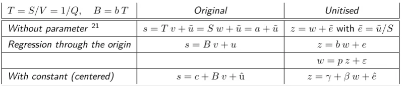
Q=V /Sis the natural quota, or number of votes to cover a seat. There may be a threshold to get a seat, or just the natural quota. Voters may vote for parties that do not pass the threshold and that thus get no seats. These votes sum to the “wasted vote”W. Standardly the wasted vote and zero seats are collected in one category “Other”, so thatv andsstill have the same length. The votes that cause a seat are V e=V₋W. For regression it is conventional to writes=T v, so thatsis explained byv. We call this vector-proportionality because of the lack of a constant. Any such relation also holds for its sum totals, and we can usefully define T =S/V = 1/Q. In reality we haves=B v+u or z=b w+ewith proportionality parameter b and errore. There is only unit proportionality or equality if z =w or b = 1 and e= 0. Leta=S v/V =T v=v/Q=S w be the proportionally accurate average of seats that a party might claim. A common error term is(s₋a) =S(z₋w). There will be at least an error from the need of integer values for seats. The valuea=Swwill be the average, and apportionment ofswill tend to be for Floor[a]_≤s_≤Ceiling[a]. The major distinctions are inTable 2.

Table 2: Basic models and their errors

T =S/V = 1/Q, B=b T Original Unitised

Without parameter 21

s=T v+ ˜u=S w+ ˜u=a+ ˜u z=w+ ˜ewithe˜= ˜u/S

Regression through the origin s=B v+u z=b w+e w=p z+ε

With constant (centered) s=c+B v+ û z=γ+β w+ ˆe

The analysis better uses regresssion through the origin (RTO) and not regression with a constant (Pearson). The unit simplex is the natural environment to look at this, though we should not forget about the role ofS. There are three different error measures:

21

[image:20.595.105.504.507.593.2]

(21)

• eˆfrom the standard regression with a constant, using centered data (Pearson).

• e from RTO, with coefficientb =z′_w/w′_{w. (SDID uses} _e.)

• e˜=z- w or the plain difference, using b= 1. (ALHID and EGID use e.)˜

Some useful mnemonics directly are:

1. eˆ′_e_ˆ_≤_e′_e_≤_e_˜′_e_˜_{because regression parameters allow the reduction of error.}

2. e picks up a potential source for proportionality that˜edoes not allow for.

3. 1′_˜_e_{= 0} _and_b_{= 1}₋₁′_e_because₁′_z_{= 1}′_w_{= 1}_.

4. b = z′_w/w′_w _{because we multiply} _z ₌ _{b w}₊_e _with _w′ _while _w′_e_{= 0}_{. The} regression selects the b with perpendicular w and e, or with w′_e _{= 0} _and minimal e′_e.

5. Taking the plain differencese˜=z₋w and weighing them by the vote shares and normalising on their squares, givesw′_e/w_˜ ′_w₌_b₋₁₍₌₋₁′_e_{from above).} Thisb= 1 +w′_e/w_˜ ′_w_{might perhaps be seen as an “implicit outcome”, though} it only works of course since we already identified b from geometry.

For centered data, we had a simple direct relation between on the one hand the Euclidean norm of the error, via SSE and RMSE, and on the other hand the sine p

1₋R2 ₌ p

SSE/SST. We now wonder about RTO. Observe that the Euclidean norm of the error is√SSE = √e′_e₌ _k_e_k _{while the Euclidean distance between the} vectors is√˜e′_e_˜₌ _k_˜_e_k ₌_k_z₋_w_k_.

4.5 Disproportionality, dispersion and education

The notion of “proportionality” derives from the notion that the seats (tens) for the parties should be proportional to the votes (millions) for the parties. A formal statement iss=T v. When we shift attention to the shares w andz then we want these proportions to beequal. We run a bit into a verbal complication when we want to see thatw andz would beproportional too.

(22)

preferable to speak about “unit or diagonal proportionality” for voting rather than “proportionality”. Only whene= 0 then we also have equality. Equal Representation is better anyway, whence we better abbreviate EPR instead of PR. It may be difficult to change a convention, but it would help for mathematics education.

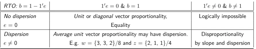
[image:22.595.106.552.321.407.2]

This calls attention to the relation with dispersion. Table 3reviews the relations. The key relationship in RTO is that b = 1₋1′_{e. Thus} _b _{= 1} _↔ ₁′_e _{= 0. The} upper right cell is impossible: Not[e = 0 & 1′_e ₆_{= 0}_{]. The lower right case of} disproportionality implies dispersion, but dispersion (e ₆= 0) need not imply such disproportionality. The middle column withb= 1 is in opposition to the right column, but we must distinguish between unit or diagonal vector-proportionality (equality) without dispersion and such average outcome with dispersion.

Table 3: Disproportionality and dispersion in Regression Trough the Origin (RTO)

RTO: b= 1−1′_e ₁′_e_{= 0}_& _b_{= 1} ₁′_e₆_{= 0}_&_b₆_{= 1}

No dispersion Unit ordiagonal vector proportionality, Logically impossible

e= 0 Equality

Dispersion Average unit vector proportionality may have dispersion. Disproportionality

e6=0 E.g. w= {3, 3, 2}/8 andz= {2, 1, 1}/4 by slope and dispersion

With b= 1 then e =z₋b w = z₋w = ˜e. We already had 1′_e_˜_{= 0} _but _b _{= 1} causes also1′_e_{= 0}_{. When} _w′₍_z₋_w_{) = 0} _then _z₋_w_{= 0}_{is only a special case.}

4.6 True variables v∗ _and s∗ _{and particular observations} v _and s

A proportional relationship for 1D variables is best described by the 2D lineλ y+µ x= 0, which coefficients may be normalised on the unit circle. For nonzeroλthis reduces toy=T xwithT =₋µ/λ, where slopeT also is the tangent of the angle of the line with the (horizontal)x₋axis. For vectors this generalises into vector-proportionality, with now a plane u = λ y+µ x and then choosing u = 0 so that y = T x again. For example,y =_{1, 2, 3_} andx=_{2, 4, 6_}, thenT = 1

2, and we would see a line without dispersion in the scatter plot.

• The notion of unit proportionality as in the liney = 1x+ 0 is a mathematical concept, while in statistics with dimensions we can rebase the variables, so that there need not be a natural base for 1.

• For voting, there are natural bases in the individuals and seats. Larger parlia-ments may have more scope for a better fit. Still, normalisation onto the unit simplex makes sense.

(23)

also holds for the totals. Thus S = 1′_s ₌ _T ₁′_v ₌ _{T V}_{. In} _{_{w, z}_} _{space it} reduces to a scatter with diagonal z = w because division gives z = s/S = T v/S =T v/(T V) =w. When any vector-proportional relationship (also non-unity) is transformed onto the unit simplex, then they become unit or diagonal proportional in the scatter, and we lose the original information.

• There also is dispersion. Vector proportionality may only holdon average. For the sake of understanding this issue of proportionality, but not for the sake of estimation and hypothesis testing, we now distinguish true elements and their observations. The basic solution namely is to distinguish on one hand the true vector-proportionality s∗ ₌ _T∗_v∗ _{that holds for all} _{true elements,} _{and on the} other hand observations (e.g. errors in variables) s= B v+u, for which we only have the definition for thesum totals asT =S/V. This also generatesu˜ from s=T v+ ˜u. For example for some v∗_{, perhaps}_s∗ ₌_a∗₌_Sw∗_.

• For the unit simplex we have z∗ ₌ _w∗ _{but for the data} _z ₌ _{w b}₊_{e. We} divided by S and took b=B V /S=B/T ande=u/S. Thus we should not focus only on parameters B and b but also be aware of the hidden Q=V /S or T = 1/Q, and perhaps consider T as an estimate onT∗_.

4.7 Cos, slope and concentrated numbers of parties (CNP)

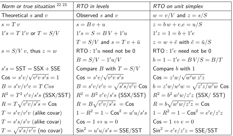
We have b =z′_w/w′_w ₌ p

z′_z/w′_w _{Cos[z, w]. The relation between Cos and} _b _is by means ofw′_w _and_z′_{z. They take the place of the covariances that are not used} in RTO, and they are also known as the Hirschman-Herfindahl concentration indices. They are known in the voting literature by the inverse “effective number of parties” NV = 1/w′w and NS = 1/z′z. Since it hasn’t been clarified what “effectiveness” would be, a better term is “concentrated number of parties” (CNP).

For theory we have s∗ ₌_T∗_v∗ _{for the}_vectors_{, but for the data we have} _s₌ _Bv +u and thus only T =S/V for the totals. Thus there are not only parameters B and b but also an “estimate” T on T∗ _{(or perhaps institutionally given} _T ₌ _T∗_).

Table4reviews the relations. For readibility we drop the stars in the theory column on the LHS.

Key points of RTO on the unit simplex are, using mostly the last column:

1. The sum of errors1′_u _or ₁′_e_{need not be 0, but}₁′_u_˜_{= 0} _and₁′_e_˜_{= 0}_.

2. It is a contribution to RTO by (seeming) compositional data that we now also look atT =S/V ands=T v+ ˜u, orz=w+ ˜e. Voting theory currently uses this, but it might be inoptimal.

3. Useful to be aware of: b w′_w ₌ _{p z}′_z ₌ _w′_z ₌ _b/N