http://www.scirp.org/journal/jamp ISSN Online: 2327-4379
ISSN Print: 2327-4352
DOI: 10.4236/jamp.2017.511177 Nov. 13, 2017 2172 Journal of Applied Mathematics and Physics
A New Job Shop Heuristic Algorithm for
Machine Scheduling Problems
Maryam Ehsaei
1, Duc T. Nguyen
21Civil and Environmental Engineering Department, Old Dominion University, Norfolk, VA, USA
2Civil and Environmental Engineering (CEE) and Modeling, Simulation and Visualization Engineering (MSVE) Departments,
Old Dominion University, Norfolk, VA, USA
Abstract
The purpose of this research is to present a straightforward and relatively effi-cient method for solving scheduling problems. A new heuristic algorithm, with the objective of minimizing the makespan, is developed and presented in this paper for job shop scheduling problems (JSP). This method determines jobs’ orders for each machine. The assessment is based on the combination of dispatching rules e.g. the “Shortest Processing Time” of each operation, the “Earliest Due Date” of each job, the “Least Tardiness” of the operations in each sequence and the “First come First Serve” idea. Also, unlike most of the heuristic algorithms, due date for each job, prescribed by the user, is consi-dered in finding the optimum schedule. A multitude of JSP problems with different features are scheduled based on this proposed algorithm. The models are also solved with Shifting Bottleneck algorithm, known as one of the most common and reliable heuristic methods. The result of comparison between the outcomes shows that when the number of jobs are less than or equal to the number of machines, the proposed algorithm concludes smaller, and better, makespan in a significantly lower computational time, which shows the supe-riority of the suggested algorithm. In addition, for a category when the num-ber of jobs are greater than the numnum-ber of machines, the suggested algorithm generates more efficient results when the ratio of the number of jobs to the number of machines is less than 2.1. However, in this category for the men-tioned ratio to be higher than 2.1, the smaller makespan could be generated by either of the methods, and the results do not follow any particular trend, hence, no general conclusions can be made for this case.
Keywords
Heuristic Algorithm, Job Shop Scheduling, Shifting Bottleneck, Makespan
How to cite this paper: Ehsaei, M. and Nguyen, D.T. (2017) A New Job Shop Heu-ristic Algorithm for Machine Scheduling Problems. Journal of Applied Mathematics and Physics, 5, 2172-2182.
https://doi.org/10.4236/jamp.2017.511177
Received: October 17, 2017 Accepted: November 10, 2017 Published: November 13, 2017
Copyright © 2017 by authors and Scientific Research Publishing Inc. This work is licensed under the Creative Commons Attribution International License (CC BY 4.0).
http://creativecommons.org/licenses/by/4.0/
DOI: 10.4236/jamp.2017.511177 2173 Journal of Applied Mathematics and Physics
1. Introduction
Job shop scheduling (JSP) has been one of the most critical subjects in optimiza-tion and applied mathematics in the past few decades. Its vast applicability in the industry and all economic domains, and on the other hand its complexity, spe-cifically for large-scale problems, make this topic very critical [1][2]. JSP is an NP-hard problem due to its computational complicacy [3] [4]. Based on the scheduling literature, a relatively small problem consists of 10 jobs and 10 ma-chines, proposed by Muth and Thompson [5], remained unsolved for more than a quarter of a century. Also, the fact that a scheduling problem included 15 jobs and 15 machines is considered unsolvable with the exact method nowadays, clearly shows the sophistication of this kind of problems [6][7].
In job shop scheduling problems “n” jobs are needed to be processed in “m” machines. Each job includes some operations, each of which are required to be done by a particular machine. Each machine only can process one job at a time and cannot be interrupted [8]. The order of jobs in each machine is calculated by minimizing a specific character. In this paper, the completion time of all jobs, which is called makespan, is the objective [9].
Lots of algorithms and procedures have been proposed for efficiently sche-duling JSP, which are divided into three major groups: 1) the exact algorithms; such as the one proposed by Giffler and Thompson (1960), and branch and bound by Lageweg, Lenstra and Rinnooy Kan (1977) [7]. This group results are surely optimum, but they are too time-consuming to reach, 2) heuristic proce-dures; such as Palmer, Johnson and Shifting Bottleneck algorithms. They are not always derived optimum answer; some gives answers close to optimum. Com-paring to two other groups, the computational time of algorithms in this catego-ry is relatively small, 3) meta-heuristic Algorithms; such as genetic algorithm, and SA and TS algorithms by Fattahi, Mehrabad and Jolai [10]. This group does not guaranty the optimal answer, but present better results comparing to the second group.
A new heuristic algorithm is presented in this paper for optimally scheduling JSP. This method is the result of combining different dispatching rules, so, its implementation is justly straightforward. It is also worth to mention that tardi-ness is the difference between the completion time of each job (or operation) and the job’s related due date (or relative due date); in other words, the time that a job takes to be completed after its due date arrives is called tardiness.
Due to the complexity of developing a reliable and efficient algorithm, some heuristic algorithms just consider operations’ processing times, ignoring the jobs’ due dates and others are designed based on the due dates and ignored the processing time. However, the new algorithm presented in this paper takes both factors into account.
DOI: 10.4236/jamp.2017.511177 2174 Journal of Applied Mathematics and Physics of machines in each job may not follow a specific order [11]. So, unlike algo-rithms like Johnson and NEH, which are only applicable and useful in flow shop problems, the proposed algorithm is capable of handling the job shop schedule as well. The new algorithm detail is described in the following section.
Among all existing heuristic algorithms, Shifting Bottleneck algorithm is one of the most well-known and reliable ones. Therefore, to evaluate the reliability of the new algorithm, its results have been compared to the Shifting Bottleneck outcomes. Scheduling models for comparison of two algorithms are JSP prob-lems. The comparison of outcomes is reported in the Results section. Finally, based on the observed results, conclusions will be made.
2. Materials and Methods
2.1. Proposed Algorithm Description
The proposed algorithm has been developed based on some primary dispatching rules including “earliest due date” of each job, “shortest processing time” of each operation, “least tardiness” of operations in each sequence and “first come first serve” idea. The theory behind using these simple rules is to create a heuristic method with a straightforward procedure to apply to JSP problems, concluding to acceptable results. The efficiency of the results comparing to other heuristic algorithms, is also contemplated. Besides, the proposed method is designed in such a way that the due dates’ values required to be specified by the user. This advantage can equip users to affect their tendency in using specific due dates in the scheduling problems.
[image:3.595.205.540.650.721.2]Moreover, the sequence of operations and their related processing times for each job are needed to be imported. Besides, the user is required to clarify the machine used for each operation. The procedures’ details of the new algorithm are being described on a small example to explain the steps thoroughly.
Table 1 shows a JSP example, consisting of 3 jobs and 3 machines. The
processing times and due dates are also specified. Each job is defined in each row of the table. Each job consists of some operations, required to be done by a par-ticular machine, which each of the operations has a deterministic processing time specified in the table. For instance, Job 1 has three operations; first opera-tion processing time is 7 minutes (instead of minutes any unit of time can be used), and it needs to be done by machine 1 (M1).
1) Step 1: The minimum value of all the provided due dates is selected and subtracted from the rest of the due dates; the result values are called relative due
Table 1.Job shop scheduling example.
DOI: 10.4236/jamp.2017.511177 2175 Journal of Applied Mathematics and Physics dates. There are two reasons for doing so: 1st reason is that this way it is not
[image:4.595.210.539.522.588.2]ne-cessary to deal with values of due dates, which might be significantly large. And the second reason is that urgency of the jobs can be compared more clearly. The results of the subtraction for the mentioned example in Table 1, is elaborated in Table 2.
[image:4.595.208.539.635.732.2]2) Step 2: The new algorithm is task wise, which means the priority is the first to be operated task in each job, which is derived from the primary rule “first come first serve”. In the mentioned example the priority is the column by the title of “1st Operation” (second column of the table). These are tasks, which are needed to be completed in their related jobs, for jobs to be able to go to the next stage. Based on the explained idea, the first tasks are considered first. If there is no ready time for an operation (best situation), its completion time will be equal to their related processing time. Therefore, for each operation, the tardiness will be equivalent to the operation’s relative due date, subtracted by the related com-pletion time or the operation processing time. The procedure is presented in
Table 3. The order of implementation will be based on the least tardiness such
that, the operation with the lowest tardiness takes place first, and the operation with the most massive tardiness will take place at last. If there is a tie-breaker, the algorithm chooses the operation based on the job orders; for example in the mentioned case, between the 1st operation of job 1 and 1st operation of job 3, the priority for the algorithm is job 1.
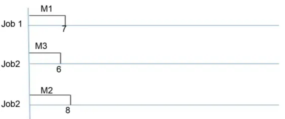
For clarification of the proposed method, execution of each step is demon-strated in a diagram, similar to Gantt chart. Gantt chart is a bar chart used to demonstrate a project schedule, which in job shop scheduling problems it usual-ly illustrates the order of jobs in each machine. However, in the diagrams used in this paper, called modified Gantt chart, the charts show the sequence of ma-chines in each job (with consideration of their order and waiting time). Figure 1
Table 2.New algorithm execution: step 1 (subtraction the value of the minimum due date
from other ones).
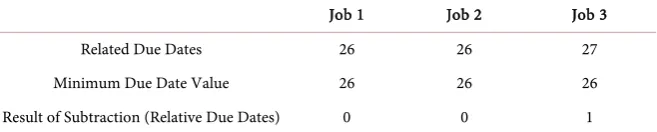
Job 1 Job 2 Job 3
Related Due Dates 26 26 27
Minimum Due Date Value 26 26 26 Result of Subtraction (Relative Due Dates) 0 0 1
Table 3.New algorithm execution: step 2 (subtraction of the relative due dates from the
completion time of each job till the end of the 1st Operations).
(Job 1, M1) (Job 2, M3) (Job 3, M2) The Least Completion Time of Each Job till
the End of the 1st Operation 7 6 8 Related Relative Due Dates 0 0 1
Result (Tardiness) 7 6 7
DOI: 10.4236/jamp.2017.511177 2176 Journal of Applied Mathematics and Physics
Figure 1.Implementation of the 1st operations on modified Gantt chart.
shows the implementation of step 2.
3) Step 3: The procedure in this step is the same as step two, just the consi-dered completion times are different. They are equal to the processing time of each job from the start of the job until the end of the current operation. For in-stance, the completion time of job 1 after the end of task 2 is equal to the sum-mation of 7 and 8 (7 + 8 = 15). Table 4 displays the detail of this step on the mentioned example. Also, the implementation of this step on modified Gantt chart is shown in Figure 2.
4) Step 4: This step is also similar to the two previous ones, by considering the completion time of each job up to the end of the current operation. The proce-dure detail and implementation on modified Gantt chart for this stage are de-scribed in Table 5 and Figure 3 consequently. Based on the modified Gantt chart it is clear that the makespan is 33.
It is also worth to mention that the completion time of all jobs (makespan) is equal to the completion time of all machines. As it is mentioned earlier the im-plementation of the operations should be in a way to avoid confliction between the machines; in other words, the ready time for each operation and the processing time of the machine before starting the current operation are needed to be considered. So, for the mentioned instance, the sequence of jobs in each machine is derived as follow:
a) M1: Job 1 − Job 2 − Job 3 b) M2: Job 3 − Job 2 − Job 1 c) M3: Job 2 − Job 1 − Job 3
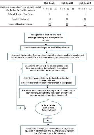
With the same procedure implemented to the mentioned example, any num-ber of jobs and machines can be scheduled by the proposed algorithm. The algo-rithm is also presented in the form of the flowchart in Figure 4.
For a new algorithm to be evaluated, it is necessary to be compared with a well-known and reliable existing algorithm in various models. One of the most popular and acceptable heuristic algorithms, which is known to be superior among heuristic algorithms for JSP, is Shifting Bottleneck algorithm proposed by Adams, Egon and Zawack [8].
2.2. Shifting Bottleneck Algorithm
DOI: 10.4236/jamp.2017.511177 2177 Journal of Applied Mathematics and Physics
[image:6.595.238.512.232.363.2]Figure 2.Implementation of the 2nd operations on modified Gantt chart.
Figure 3.Implementation of the 3rd operations on modified Gantt chart.
Table 4.New algorithm execution: step 3 (subtraction of the relative due dates from the
completion time of each job till the end of the 2nd Operations).
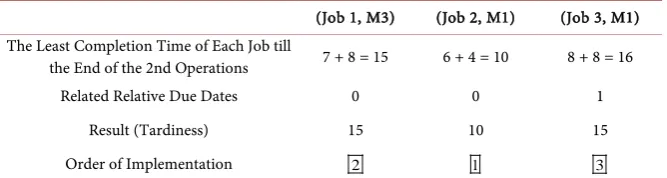
(Job 1, M3) (Job 2, M1) (Job 3, M1) The Least Completion Time of Each Job till
the End of the 2nd Operations 7 + 8 = 15 6 + 4 = 10 8 + 8 = 16 Related Relative Due Dates 0 0 1
Result (Tardiness) 15 10 15
Order of Implementation 2 1 3
promising, especially on benchmark problem sets from the literature, such that lots of researchers like, Dauzere-Peres and Lasserre (1993) and Schutten (1995), consider it as a fundamental algorithm for their work. However, the efficiency of this algorithm may be reduced by increament of the ratio of number of ma-chines per number of jobs [12].
Shifting bottleneck algorithm approach is machine wise. It is solved a one- machine scheduling problem at a time for all not sequenced machines. Then based on the rank of scheduled machines, it sets the job sequence for the highest rank machine and reorders the job sequence for others. This method is chosen for comparison with the new proposed algorithm in this paper.
3. Results
[image:6.595.207.541.426.515.2]DOI: 10.4236/jamp.2017.511177 2178 Journal of Applied Mathematics and Physics
Table 5.New algorithm execution: step 4 (subtraction of the relative due dates from the
completion time of each job till the end of the 3rd operations).
(Job 1, M3) (Job 2, M1) (Job 3, M1) The Least Completion Time of Each Job till
the End of the 3rd Operations 7 + 8 + 10 = 25 6 + 4 +12 = 22 8 + 8 + 7 = 23 Related Relative Due Dates 0 0 1
Result (Tardiness) 25 22 22
Order of Implementation 3 1 2
Figure 4.Flow chart of the proposed algorithm.
DOI: 10.4236/jamp.2017.511177 2179 Journal of Applied Mathematics and Physics 6 is allocated to the models with the same number of jobs and machines. Table 7 is associated with the models with the higher number of machines. Finally, the models with the higher number of jobs are presented in Table 8.
[image:8.595.57.539.255.479.2]Since the proposed algorithm gets advantage of the assigned due dates in the calculation of the makespan, changing them may result in varying the outcomes consequently. However, the Shifting Bottleneck algorithm does not consider the due dates provided by users, so its results will remain unchanged. In each model 27 different cases, with a set of randomly generated due dates, have been scruti-nized. For each model, the results derived by the new algorithm in all the cases have been compared to the ones derived from the Shifting Bottleneck algorithm,
Table 6.Comparison of the models with equal number of jobs and machines.
# Jobs* #Machines (Models)
Percentage of the Times that the New Algorithm Gives a Lower Makespan in 27 Iterations (%)
Makespan derived by Shifting Bottleneck
Algorithm
Makespan derived by the New Algorithm (Average of 27 Iteration
Results)
Average Computational Time for Shifting Bottleneck
Algorithm (Second)
Average Computational Time for New Algorithm
(Second)
3 * 3 88% 37 36.37037 0.061752 0.034239
10 * 10 100% 182 123.4615 0.246965 0.040610
18 * 18 100% 1489 1134.778 1.401769 0.728196
26 * 26 100% 2659 1837.185 2.556270 0.762216
35 * 35 100% 1753 1194.111 5.444633 0.842263
60 * 60 100% 3465 2605.37 37.439974 0.926187
73 * 73 100% 4143 3254.704 79.510854 1.146496 80 * 80 100% 8982 7040.077 100.277707 1.230148 100 * 100 100% 4143 3378.296 282.844018 1.662978
140 * 140 100% 6063 4822 1129.604031 4.566296
Table 7.Comparison of the models with higher number of machines.
# Jobs *#Machines
(Models)
Percentage of the Times that the New Algorithm Gives a Lower Makespan
in 27 Iterations (%)
Makespan derived by Shifting Bottleneck
Algorithm
Makespan derived by the New Algorithm
(Average of 27 Iteration Results)
Average Computational Time for Shifting Bottleneck Algorithm
(Second)
Average Computational Time for New Algorithm
(Second)
3 * 5 100% 383 231 0.754168 0.700745
4 * 10 100% 806 426.5926 0.984952 0.722524
12 * 17 100% 1423 896.5926 1.362245 0.723708
15 * 35 100% 4522 2318.704 2.888122 0.994421
12 * 60 100% 4492 2260.741 8.422953 0.706465
40 * 100 100% 12,593 7095.148 95.288633 0.994421 50 * 70 100% 11,040 7723.593 42.723094 0.922766
60 * 73 100% 7036 5024.593 66.844959 1.028324
[image:8.595.55.540.513.726.2]DOI: 10.4236/jamp.2017.511177 2180 Journal of Applied Mathematics and Physics
Table 8.Comparison of the models with higher number of jobs.
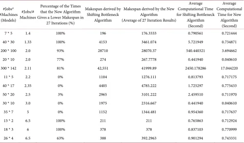
#Jobs* #Machines
(Models)
#Jobs/# Machines
Percentage of the Times that the New Algorithm Gives a Lower Makespan in
27 Iterations (%)
Makespan derived by Shifting Bottleneck
Algorithm
Makespan derived by the New Algorithm
(Average of 27 Iteration Results)
Average Computational Time for Shifting Bottleneck
Algorithm (Second)
Average Computational
Time for New Algorithm
(Second)
7 * 5 1.4 100% 196 176.3333 0.790561 0.721444
40 * 30 1.33 100% 4153 3461.074 5.721949 0.734871 200 * 100 2.0 93% 28710 28070.37 540.440321 3.694662
20 * 10 2.0 77% 274 267.7778 0.441940 0.040610
300 * 142 2.11 81% 42,551 41999.89 2450.178286 17.044220
11 * 5 2.2 0% 1104 1276.111 0.813793 0.717175
40 * 17 2.35 0% 4405 4785.222 1.725297 0.775433
50 * 20 2.5 3% 2965 3101.222 2.459510 0.711970
30 * 10 3.0 0% 1975 2316.667 0.441940 0.040610
35 * 7 5 0% 1152 1344.481 0.954360 0.717637
13 * 2 6.5 100% 211 211 0.765863 0.712924
18 * 3 6 100% 378 378 0.837103 0.770999
26 * 4 6.5 63% 388 392.2963 0.901294 0.743331
but to save the space, for each model, just the average of the results of 27 states is presented here. The percentage of the number of the times that the new algo-rithm produces lower makespan is also reported here. Therefore, for each group of problems two algorithms have been compared 270 times or more. The obser-vation from the compared models is noted in this section. It is worth to mention that all the considered processing times are chosen randomly.
As it is shown in Table 6, the new algorithm produces lower makespan in al-most all iterations. Moreover, it is observed that by increasing the size of the problem in this category (number of jobs and machines) the difference, between the computational time generated by the two algorithms becomes significant. Growing the problem size is also concluded to the variation of makespans, pro-duced by two methods for an identical problem, to be increased considerably.
When the number of machines is higher than the number of jobs in all cases the derived makesspan by the proposed method is lower than the identical ones derived from the Shifting Bottleneck algorithm. The difference between the computational time is also increased by the increment of the size of the problem. The details are presented in Table 7.
DOI: 10.4236/jamp.2017.511177 2181 Journal of Applied Mathematics and Physics lower makespan, in a smaller computational time. However, when the men-tioned ratio is higher than 2.2, the observed results do not have solidarity, which means in some situations the proposed algorithm, and in some other cases Shifting Bottleneck algorithm, generates lower makespan.
4. Conclusions
A new algorithm for scheduling job shop problems has been proposed in this ar-ticle. This algorithm is based on the combination of some primary dispatching rules like the “Shortest Processing Time” of each operation, the “Earliest Due Date” of each job, the “Least Tardiness” of the operations in each sequence and the “First come First Serve” idea. Straightforward procedures and ease of im-plementation are two of the most significant advantages of the proposed me-thod. The flowchart and the execution steps have been described in previous sections in detail.
For numerical evaluation and verification of the suggested method, its pro-duced results have been compared to the outcomes derived by the Shifting Bot-tleneck algorithm for enormous problems. Results comparison is presented in this paper for more than 30 models with almost 900 different iterations (using random due dates).
Based on the compared models, it is observed that when the number of jobs is less than or equal to the number of machines, the proposed algorithm produces lower makespan in a significantly smaller computational time, which shows the superiority of the proposed method. Also, the larger the size of the problem, the more the difference between the identical makespans generated by two methods. Besides, in the mentioned categories, in the models with a larger size for an identical problem, the computational time by the new method is remarkably less than the computational time by the Shifting Bottleneck algorithm.
It is also observed that when the ratio of the number of jobs to the number of machines, is less than 2.1, the proposed algorithm produces lower makespan in a smaller computational time. But, when the mentioned ratio becomes greater than 2.1, the smaller makespan could be generated by either of the methods, and the results do not follow any particular trend, hence, no general conclusions can be made for this case.
It is also perceived that for all the tested cases, the computational period of the proposed method is lower than the computational time of the Shifting Bottle-neck algorithm.
Acknowledgements
Authors would like to thank Old Dominion University for providing resources to facilitate this project.
References
DOI: 10.4236/jamp.2017.511177 2182 Journal of Applied Mathematics and Physics
[2] Nguyen, S., Zhang, M., Johnston, M. and Tan, K.C. (2012) Evolving Reusable Oper-ation-Based Due-Date Assignment Models for Job Shop Scheduling with Genetic Programming. European Conference on Genetic Programming, Malaga, 11-13 April 2012, 121-133.https://doi.org/10.1007/978-3-642-29139-5_11
[3] Zhang, R. and Wu, C. (2011) An Artificial Bee Colony Algorithm for the Job Shop Scheduling Problem with Random Processing Times. Entropy, 13, 1708-1729. https://doi.org/10.3390/e13091708
[4] Brucker, P., Jurisch, B. and Sievers, B. (1994) A Branch and Bound Algorithm for the Job-Shop Scheduling Problem. Discrete Applied Mathematics, 49, 107-127. https://doi.org/10.1016/0166-218X(94)90204-6
[5] Muth, J.F. and Thompson, G.L. (1963) Industrial Scheduling. Prentice-Hall, Engle-wood Cliffs, N.J.
[6] Zhang, C.Y., Li, P., Rao, Y. and Guan, Z. (2008) A Very Fast TS/SA Algorithm for the Job Shop Scheduling Problem. Computers & Operations Research, 35, 282-294. https://doi.org/10.1016/j.cor.2006.02.024
[7] Lageweg, B.J., Lenstra, J.K. and Rinnooy Kan, A.H.G. (1978) A General Bounding Scheme for the Permutation Flow-Shop Problem. OPNS RES,26, 53-67.
https://doi.org/10.1287/opre.26.1.53
[8] Adams, J., Egon, B. and Zawack, D. (1988) The Shifting Bottleneck Procedure for Job Shop Scheduling. Management Science, 34, 391-401.
https://doi.org/10.1287/mnsc.34.3.391
[9] Bhosale, P.P. and Kalshetty, Y.R. (2016) Genetic Algorithm for Job Shop Schedul-ing. International Journal of Innovations in Engineering and Technology (IJIET), 7, 357-361.
[10] Fattahi, P., Mehrabad, M.S. and Jolai, F. (2007) Mathematical Modeling and Heu-ristic Approaches to Flexible Job Shop Scheduling Problems. Journal of intelligent manufacturing, 18, 331-342. https://doi.org/10.1007/s10845-007-0026-8
[11] Abbas, M., Abbas, A. and Khan, W.A. (2016) Scheduling Job Shop—A Case Study.
IOP Conference Series: Material Science and Engineering, 146, 021052. https://doi.org/10.1088/1757-899X/146/1/012052