Dynamic Conditional Correlation between Electricity, Energy (Commodity) and Financial Markets during the Financial Crisis in Greece

ISSN Online: 2162-2442 ISSN Print: 2162-2434

DOI: 10.4236/jmf.2017.74055 Nov. 29, 2017 990 Journal of Mathematical Finance

Dynamic Conditional Correlation between

Electricity

,

Energy (Commodity) and Financial

Markets during the Financial Crisis in Greece

Panagiotis G. Papaioannou

1

,

George P. Papaioannou

2,3

,

Akylas Stratigakos

4

,

Christos Dikaiakos

2

1_{Applied Mathematics and Physical Sciences, National Technical University of Athens, Athens, Greece}

2_{Research, Technology & Development Department, Independent Power Transmission Operator (IPTO) S.A., Athens, Greece} 3_{Center for Research and Applications in Nonlinear Systems (CRANS), Department of Mathematics, University of Patras, Patras,}

Greece

4_{Department of Electrical and Computer Engineering, University of Patras, Patras, Greece}

Abstract

Liberalization of electricity markets has increasingly created the need for un-derstanding the volatility and correlation structure between electricity, finan-cial and energy commodity markets. This work reveals the existence of struc-tural changes in correlation patterns among these markets and links the changes to both fundamentals and regulatory conditions prevailing in the markets, as well as the current European financial crisis. We apply a Dynamic Conditional Correlation (DCC) GARCH model to a set of market’s funda-mental variables, related commodity markets and Greece’s financial market and microeconomic indexes to study their interaction. Emphasis is given on the period of severe financial crisis of the Country to understand “contagion” and volatility spillover between these markets. This approach enables us to capture the changing co-movement of assets within and between markets (fi-nancial, commodity, electricity) as market conditions change. The main re-sults are that there is strong evidence of volatility spillover (or co-volatility) between financial and commodity market, while the Greek electricity market seems to be almost “isolated” from these two markets.

Keywords

Dynamic Conditional Correlation, Garch, Electricity & Financial Markets

1. Introduction

In the financial and Commodity markets, conditional volatility models have found an extensive application. However the studies focusing on modeling the How to cite this paper: Papaioannou, P.G.,

Papaioannou, G.P., Stratigakos, A. and Dikaiakos, C. (2017) Dynamic Conditional Correlation between Electricity, Energy (Commodity) and Financial Markets during the Financial Crisis in Greece. Journal of Mathematical Finance, 7, 990-1033. https://doi.org/10.4236/jmf.2017.74055 Received: September 12, 2017 Accepted: November 26, 2017 Published: November 29, 2017

Copyright © 2017 by authors and Scientific Research Publishing Inc. This work is licensed under the Creative Commons Attribution International License (CC BY 4.0).

http://creativecommons.org/licenses/by/4.0/

DOI: 10.4236/jmf.2017.74055 991 Journal of Mathematical Finance spillover of price conditional volatility between financial, energy (commodity) and wholesale electricity markets in Europe are very few. We provide first a brief literature review.

The transmission of price volatilities between two natural gas markets, the British and Belgium ones, is investigated by Bermejo-Apricio et al., (2008) [1]. They applied GARCH (1,1) and EGARCH (1,1) for the univariate case and a DCC and BEKK (named after Baba, Engle, Kraft and Kroner, Engle, R. F. et al. 1995 [2]) for the bivariate case, on deseasonalized daily prices of National Ba-lancing Point (NBP) and Zeebrugge Hubs. They took also into consideration the Interconnector gas pipeline’s used capacity as an exogenous variable for the conditional variance. Their study has shown the existence of an inverse leverage effect for the Zeebrugge and NBP prices i.e. large price increases (positive shock) increase the conditional volatility more than large price drops (negative shock). The main conclusion in their paper is that the Interconnector gas pipeline im-pacts strongly the conditional variance of NBP and Zeebrugge, resulting in an increase of the volatility linkage between the two markets when 50% or more of the pipeline’s total capacity is used.

The interaction between gas spot prices at Zeebrugge, one month-ahead Brent Oil Prices and temperature, for period 2000-2005, is examined in the work of Regnard and Zokoian (2011) [3]. They used a Vector Error Correction Model (VECM) to investigate the joint dynamics of the three variables and found (us-ing Johansen’s approach) evidence of a cointegrat(us-ing linkage between the three variables. Also, using an asymmetric Constant Conditional Correlation (A-CCC) model and multivariate GARCH have shown that volatilities of the three series are dependent on their own lagged volatilities. They found significant cross-effects in the conditional correlation matrix. They also examine the influence of 3 dif-ferent temperature regimes on the conditional variance (low temperature regime positive shocks increase the conditional variance, while the Zeebrugge price’s volatility is increased due to negative shocks originating from high temperature regime).

The interaction between Brent Oil and NBP spot price returns is estimated by Asche et al. (2009) [4], conducting a multivariate GARCH and a BEEK model. They show that prior to 2003 (a year corresponding to a breakdown), there is not any impact of shocks occurred in the oil (gas) market on the conditional va-riance of gas (oil). They argue that a possible explanation of the impacts of oil price shocks on the volatility of gas prices is the small or limited available capac-ity of the European gas market infrastructure as well as the enhanced levels of maturity and liquidity of the European NG spot market.

DOI: 10.4236/jmf.2017.74055 992 Journal of Mathematical Finance [5] paper, while front month prices for Brent Oil and Natural Gas (NG) are used in the Mansanet-Bataller-Soriano’s (2009) [6] paper. Trivariate multivariate GARCH models, namely the CCC, DCC and the BEEK model were used to “capture” the volatility spillovers in Chevallier’s (2012) [5] work, while a BEEK model is used in the case of the other paper. The DCC model used in Cheval-lier’s work shows that the conditional correlation between Oil and NG is from −0.3 to 0.3 and for NG and CO2 is from −0.2 to over 0.1.

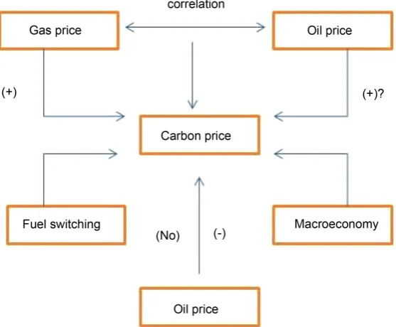
Commodity prices i.e. gas, oil, coal as well as electricity have a strong effect in the determination of Carbon prices, in Phase I of the EU ETS, as shown in the papers of Mansanet-Bataller et al. (2011) [7], Alberola et al. (2008) [8], and Hin-termann (2010) [9]. Positive impact on EUA prices is shown to have gas and oil prices. However, the positive impact of Oil prices is ambiguous because this in-fluence may be also attributed to fuel switching effect, to the correlation be-tween oil price and overall macroeconomic conditions or to the Oil-gas price correlation (Rickels et al., 2010) [10]. These above interdependencies are shown in the following simple “causal map” (Figure 1).

Yearly compliance events combined with Regulatory (institutional) and the macroeconomic uncertainties in EUA market have a strong influence on dy-namic development of EUA price volatility (Chevallier, 2011a) [11]. In the same work, no evidence was found on the effect of the financial crisis in 2008 on the Carbon price volatility.

[image:3.595.236.515.457.687.2]

Bredin and Muckley (2011) [12], using a cointegration approach, have found an equilibrium linkage (in a new price regime in Phase II) between Carbon fu-tures prices and Energy prices. The main conclusion from this work is that in

DOI: 10.4236/jmf.2017.74055 993 Journal of Mathematical Finance Phase II the Carbon-energy Co-movement is reinforced, in parallel with a structural increase in correlation patterns.

Another group of literature is concentrated on the mutual interactions be-tween Carbon and Energy market, considering the bi-directional influence. By using a cointegrated VAR method, Bunn and Fezzi (2009) [13] report that gas price affects the EUA price and both jointly affect the equilibrium price of elec-tricity in the UK market. In opposite direction are the results of Nazifi and Mi-lunovich (2010) [14]. They instead found just short-run linkages (s.r.l) between Carbon and Oil, Carbon and gas, and electricity and Carbon, and no long-run relationship between Carbon, energy and electricity prices (shown in Figure 2).

Granger causality tests were performed by Keppler and Mansanet-Bataller (2010) [15], and found that during Phase II, electricity prices Granger cause Carbon prices.

Volatility spillover between Carbon and Energy was examined by Mansa-net-Bataller and Soriano (2009) [6] using a BEKK-GARCH model. They found that Carbon volatility is directly and indirectly (via covariance) affected by the Oil and natural gas volatility. Carbon volatility is also affected by shocks com-ing from Carbon and Oil markets.

Moreover, Koch, N. (2014) [16] has studied the dynamic linkages among Carbon (European Union Allowances, EUA), Commodity (Energy) and finan-cial markets using the Smooth Transition Conditional Correlation (STCC) ap-proach, an extension of DCC model. He calls Oil, gas, coal, electricity, stocks and bonds as accepted fundamentals. He used time as transition variable to allow for structural breaks related to institutional changes in the European Union Emissions Trading System (EU ETS). His main conclusion is that correlation depends on market uncertain conditions, reflecting the connection between Carbon and Financial markets due to common macroeconomic shocks hap-pened over the 2008/09 financial crisis.

[image:4.595.222.524.578.692.2]

The linkage between EUA and Financial markets as described in Koch’s [16] work serves as a firm basis on which we build our work. The component “EUA-financial and electricity markets linkage” or more precisely the volatility spillover between eua-financial markets, is depicted in the following triplet “causal map” (Figure 3).

DOI: 10.4236/jmf.2017.74055 994 Journal of Mathematical Finance Figure 3. Interdependence between the financial, energy and electricity markets.

We share Koch’s [16] argument on the existence of correlation asymmetries due to time-varying market uncertain conditions and examine in our work here the influences of these conditions on the dynamic conditional correlations dur-ing periods of calmness and turmoil in financial markets. This is of particular value in the case of Greece, a State hit heavily by two crisis, the financial one 2008-2009 and the Greek Debt (Sovereignty) crisis started in late 2010.

We must note that in this study, we refer as “financial crisis” to the Subprime mortgage crisis, which spans from 2008 to late 2009 in our sample, and as “Greek debt crisis” to the European sovereign debt crisis of late 2009.

The rest of the paper is organized as follows. In Section 2 we describe the ma-croeconomic risk factors and stretch the significance of volatility spillover or co-movement, between 3 different markets: financial, energy commodity and Power (electricity) markets. The used data sets and a short description of the Greek electricity market and financial market are given in Section 3. Section 4 provides all necessary information on the methodology (DCC, CCC etc) used in this work and finally the empirical findings are presented in Section 5 followed by Conclusions in Section 6.

2. Macroeconomic Risk Factors and the Significance of

Volatility Spillover or Co-Movement

[image:5.595.234.514.74.171.2]

eco-DOI: 10.4236/jmf.2017.74055 995 Journal of Mathematical Finance nomic “climate”.

2.1. The Importance of Input Fuel Prices Volatilities and

Their Co-Movement with EUA

The operational behavior that links fuel and EUA is the generator’s fuel-switching. This is so because a higher gas (coal) price ends up to a higher (lower) eua:

ngasUK then eua coal then eua

↑ ↑

↑ ↑

This observation is a good theoretical basis for explaining the co-movement or the Dynamic Conditional Correlation between input fuel prices and eua. A pro-ducer of electric power uses hydrocarbon fuels and eua as production inputs, so he depends on these “assets”. This situation is not the same as in a financial market in which a portfolio manager can diversify his assets portfolio by altering the (percentage) share of the assets, in order to protect the value of the portfolio from price changes (hedging). The power producer is exposed to changes in prices in electricity, energy (commodity) and EUA markets. Therefore, the risk-averse Power Plant Owner (producer) has to operate in forward (futures) markets for hedging his profits against the risk of unpredictable and unfavorable price volatility. In other words he tries to lock in a given profit based on a given (assumed) marginal generation cost.

However, the key variables in a futures market are the price volatility of an “asset” (input fuel, eua etc.) and its co-movement with other relevant asset’s price. This co-movement is measured by its conditional covariance or correla-tion price volatility is usually expressed as condicorrela-tional variance.

Following Koening, P. (2011) [20], in order to realize how a Power Producer is exposed to eua and fuel price co-movements, we recall the marginal genera-tion Cost MCi, in €/GJe of generating a given unit of power, by using as input fuel i:

i i i i i FC EF MC EC n n

= + ₍₁₎

where FCi is the fuel cost in €/GJ, ni is the power plant net thermal efficiency in GJe/GJ (GJe is the power output in gigajoule of electricity, GJ the power input in gigajoule of fuel), EFi the Green House Gas (GHG) emission factor in kg CO2/GJ and EC is the GHG emission cost in €/kg CO2. Equation (1) is actually a simplification and MCi is primarily estimated by the variable costs of fuel and CO2.

The variance of MCi is given by (Koening, P., 2011) [20] 2

2 2 2

,

2 2

1 1

2

i i i i

i i

MC FC EC FC EC FC EC

i i

i i

EF EF

n n

n n

σ = σ + σ + ρ σ σ ₍₂₎

where ρFC ECi, is the correlation of input fuels and eua and 2

i

σ _{are variances.}

DOI: 10.4236/jmf.2017.74055 996 Journal of Mathematical Finance will examine how the volatility in Energy commodity markets in combination with volatility in financial markets affect the above conditional correlations.

2.2. The Correlation of Carbon Emission Allowances (Eua) with

Other Commodity Prices (NgasUK

,

Brent

,

Coal or Lignite)

The optimal merit order of power generation is affected by changes in the rela-tive price of input fuels. These changes ultimately result in a fuel-switch, by the power generator which tries to maximize its profit. Fuel-switching is not an ob-servable operational variable and has to be inferred from changes occurred in the relative marginal costs.

From the above we conclude that the unobserved fuel-switching behavior by generators is the main factor of “producing” the correlation between input fuels (brent, ngasUK) and carbon emission allowances (eua). The empirical Carbon price moves between two extreme values, the upper bound theoretical switch price SPu defined as the price of CO2 above which natural gas is the preferred input fuel (technology), no matter what the thermal characteristics of the gener-ation mix (or plant portfolio) (Koening, P., 2011) [20]. SPu is given by

E I

coal gas gas coal

u I E E I

gas coal coal gas

n FC n FC

SP

n EF n EF

− =

− (3)

where E coal

n and EF_coalE are the thermal efficiency and emission factor of the most efficient coal fired power plant in a Country’s generation mix (plant portfolio). The thermal efficiency and emission factor of the most inefficient gas fired power plant are I

gas

n , EF_gasI respectively. Therefore, if the price of carbon increases then it will motivate generators to switch input fuels from Coal (Lignite) to gas. As soon as CO2 price has attained SPu, even generators that have a choice between the most inefficient gas and most efficient Coal plant, will have, at the end, to “move” to natural gas generation. So, there is no other technology feasible generation mix which prefers coal over gas genera-tion. An electricity producer, a profit maximizing “rational” market player, will switch generation from using Coal (lignite) to using natural gas, just in the case of the empirical emission price exceeds the SPu.

The lower bound theoretical switch price, SPl, is the price of Carbon below which Coal is the preferred input fuel, irrespective of the thermal characteristics of the generation mix (Koening, P., 2011) [20].

I E

coal gas gas coal

l E I I E

gas coal coal gas

n FC n FC

SP

n EF n EF

− =

− (4)

where n_coalI ,EF_coalI the thermal efficiency and emission factor, respectively, of the most inefficient coal fired plant in a Country’s generation mix. E

gas

n and

E gas

EF are the thermal efficiency and emission factor, respectively, of the most efficient natural gas fired plant in the Country’s generation mix.

DOI: 10.4236/jmf.2017.74055 997 Journal of Mathematical Finance price reaches SPl, all generation “players” will have to switch to Coal, even though they have the choice between the most inefficient Coal and the most ef-ficient natural gas plant.

From the above, the main conclusion is that a higher share of Coal production (Lignite in the case of Greece), rationally, will increase the demand for Carbon emission allowances (eua) and its price will go upwards again.

Combining all the above the empirically observed EUA (eua time series) is expected to move between the two time-varying extreme values, SPl and SPu. From the definitions given by (3) and (4), two correlation regimes are possible between eua and other commodities (ngasUK, Brent, Coal, Lignite). The first is when eua (empirical carbon price) either exceeds SPu or falls below SPl, a situa-tion referred as Static merit order. In this case either natural gas or Coal is clearly the preferred input fuels and small changes in their prices do not change the merit order. In this case there is no financial motivation to switch input fu-els, which results in an unchanged demand for eua and eua therefore fuel prices are decoupled. The second correlation regime is when eua is between SPl and

SPu.

Here we have a mixed merit order in which there is no clear ranking of the input fuels in the merit order and the crucial now factor in choosing one of the two fuels is their thermal efficiencies. This is a situation where small fuel price changes have a strong influence in the merit order, which in turn result in changes of demand for eua. This fuel and eua prices are coupled (or co-move). The coupling and decoupling of eua and fuel prices have been studied in depth by Koening P. (Koening, P., 2011 [20]). A very important conclusion from his work is that if in a period t the relative forward (futures) fuel and eua prices are in such levels that make a constant merit order, then these prices are decoupled,

exhibiting a low correlation. The above situation calls for an alternative hedging strategy for securing a profit one month ahead, in comparison with a situation with coupled prices and strong correlation.

In theory, the equilibrium allowance price is equal to the marginal abatement costs incurred to reduce one ton of pollutant (Springer, 2003) [21]. The papers by Rubin (1996) [22] and Tietenber (2006) [23] describe the theoretical basis of deterministic equilibrium models and the solution, in a cap-and-trade frame-work, of the firm’s pollution cost optimization problem. Thus, the participants of the market take only these measures whose costs are less than or equal to the EUA price. The theoretical justification of linking Carbon and Commodity (Energy) markets lies in the difficulty to find proxies for the emission abatement costs of a firm and their availability.

DOI: 10.4236/jmf.2017.74055 998 Journal of Mathematical Finance [25]. Therefore, it is expected that input fuel prices and Carbon prices must be correlated, according to the requirement of an efficient market.

2.3. The Interaction of Financial and EUA Markets

Koch, N. (2014) [16] has found that EUA and financial markets are not isolated. Rather, financial market conditions impact strongly the correlations and the vstoxx index serves as an informative state variable reflecting the risk of “genet-ic” financial turmoils related to extreme events in the stock markets. According to Koch, N. (2014) [16], the correlation between EUA Stock and Bonds (eua, ase, gbonds in our case) is expected to be strongly affected by an expected high vola-tility. The correlation fluctuates upwards (downwards) with peaks reverting around the collapse of Lehman Brother. He also found an impressive commo-nality in the EUA-Brent and EUA-Stock time-varying linkages, indicating that the positive impact of Brent Oil is possibly due to the interaction of Brent Oil prices and the overall macroeconomic situation and not due to the fuel switch-ing (see below) or Oil-Natural gas correlation.

It is well known that macroeconomic conditions (economic growth) affect heavily both EUA and financial markets. An increased demand and raised dustrial production is the result of high economic activity, which in turn in-creases Carbon emissions therefore inin-creases EUA (Ellerman and Buchner, 2008) [26]. Alberola et al. (2009) [27] provide evidence of a moderate effect of Industrial production on EUA prices. Considering the Stock index as a “physi-cal” economic indicator, Hintermann (2010) [9] has found no significant influ-ence of Stock Index on EUA prices in Phase I of the EU ETS, while Bonacina et al. (2009) [28] confirm that there is a correlation between EUA prices and Euro Stoxx 50 (stoxx) in the first trading year of Phase II. Chevallier (2009) [10] document that some particular economic factors like default spread, dividend yield or short-term interest rate are weakly correlated with EUA price, although these factors have a good forecasting power in Stock, Bond and commodity markets. Such common influences on the EUA market are not evident as Bes-sembinder and Chan (1992) [29] have also observed. Furthermore, Daskalakis et al. (2009) [30] provides strong evidence on significant negative unconditional correlations between EUA and Stock markets during 2005-2007. On the oppo-site, Gronwald et al. (2011) [31] provide a strong positive Carbon-Stock markets dependence, which is higher for Brent Oil and Natural gas, by using Copula analysis. The impact of financial market turmoil on EUA market correlation with Stock price indices is assessed in the paper by Kanamura (2010) [32]. A multivariate correlation model was applied and provided evidence of an in-creased correlation in times of stock market plunge, called also contagion. The paper also suggests a reduction in correlation during the oversupply event, oc-curred in April 2006.

Carbon and Financial Markets

in-DOI: 10.4236/jmf.2017.74055 999 Journal of Mathematical Finance fluenced heavily be macroeconomic variables, and that the supply and demand of allowances is the main mechanism setting the equilibrium prices.

On the other hand, Borak et al. (2006) [33], Benz and Truck (2006) [34] con-sider Carbon as a “new” input production variable that increases the cost of generation therefore exerting pressure and uncertainties on the profits thus on the Stock market as well. They argue that EUA and Stock exhibit an indirect correlation.

The Stock market effect of the EU ETS is examined also by Veith et al. (2009) [35] and surprisingly they identified a positive correlation between EUA prices and Stock price returns of “big” European Utilities.

The way with which the inclusion of EUAs in an assets portfolio improves the investment opportunity is examined by Mansanet-Bataller (2011) [7] in which he finds that the opportunity set does not vary with the inclusion of Phase II EUAs, a result opposed to the one found by Chevallier, J. (2009b) [36]. It is shown, furthermore, in the above two latter papers that EUA returns are slightly negative and statistically non-significantly correlated with fixed-income securi-ties (like Government Bonds). This result in combination with Koch, N. (2014) [16] results is our motivation to include the Greek Government Bonds in this study, using a DCC model as opposed to the CCC models used in Mansa-net-Bataller and Chevallier papers.

2.4. The Interaction between CO

2

and Electricity Prices

Low electricity prices encourage higher electricity consumption, resulting in higher CO2 emissions. Therefore the demand for allowances may increase in case electricity utilities are not in compliance with their initial allocation, a fact that in turn exerts strong pressure of the EUA markets. A further consequence is that the increase in CO2 prices and generation costs may increase electricity prices creating the need for a demand adjustment, which of course implies some level of price elasticity.

Observed power and CO2 prices are influenced also by fuel prices. If the prices of natural gas are increased then there is a strong incentive for generating base-load electricity by using more Coal—or Lignite fired-Plants, driving up, in turn, the demand for CO2 allowances. It is worth to mention here that Coal-fired generating units emit almost twice as much CO2 as natural gas generating units. If the situation just described is sustained and the supply of allowances is not adequate, CO2 prices may increase at a level that result in a fuel switch i.e. natu-ral gas, a cleaner fuel. This “cause and effect” relationship has predicted a lot of the early CO2 price volatility due to the switching from Coal (Lignite) to gas. Using the cointegration approach, Bunn and Fezzi (2007) [13] have analyzed the impact of EU ETS on electricity and gas prices.

3. The Data Sets

DOI: 10.4236/jmf.2017.74055 1000 Journal of Mathematical Finance 2014, a total of 2160 observations. The analysis period is divided into 2 periods: a) the Subprime Crisis period (from April 2008 until the end of 2009) and b) the Greek Government Debt Crisis (early 2010 until April 4, 2011). The two periods correspond to the two shaded areas in the DCC plots (Section 5.2). The chosen sampling frequency produce sufficient number of data required to measure the dynamics of correlations which may vary due to periods of financial turmoil of differing durations. The price data are denominated in the local cur-rency of each market. To enhance our choice of data frequency, we point out that from an EU ETS participant point of view, caring for his risk management, high frequency (here daily) correlations are more useful that long-term correla-tions. The data sets are obtained from various resources, Athens Stock Exchange (ASE), Independent Power Transmission Operator (IPTO), Intercontinental Exchange (ICE) Futures Europe, Energy Information Administration (EIA) and Bloomberg.

3.1. The Carbon Market and the EUA Data

The three phases of the EU ETS, corresponding to the three compliance periods are Phase I: 2005-2007, Phase II: 2008-2012 and Phase III: 2013-2020. The pilot period of the EU ETS is the well-known to market participants Phase I. The Na-tional Allocation Plans (NAPs) determine the overall emission cap for Phase I and Phase II. Each member state determines its NAP, defining actually the total permits and the allocation mode. NAPs are approved by European Commission (EC), which settles the overall cap. Because neither borrowing nor banking of EUA (EU Allowances) were allowed between Phase I and Phase II, the price for EUAs (series eua in this paper) issued for Phase I collapsed. The first informa-tion regarding the actual EUAs released in April 2006, however the market par-ticipants considered that the total emission cap for Phase I was not restrictive. Phases II and III are linked by banking, where the transactions of spare EUAs enlarges the time period considered by the agents when they shape their expec-tations about the overall shortage of EUAs. The Banking involvement reduces, therefore, the risk of an extreme collapse of the EUA price. But, if shocks happen they still can generate strong price and volatility fluctuations. Highly efficient EUA spot and derivative markets have evolved since 2005 and the most liquid derivative market is the European Climate Exchange (ICE/ECX, London), where 90% of the futures contracts are traded.

Description of the Data

DOI: 10.4236/jmf.2017.74055 1001 Journal of Mathematical Finance day the series changes again into the next yearly contract. According to Koch (2014) [16] this method of constructing the continuous EUA series is unlikely to introduce a bias because the used futures contracts are not redeemable in Phase I. This choice in forming the EUA series is further enhanced by the fact that EUA are required only once a year, for the reason of compliance, so holding spot EUAs does not offer any advantage in comparison with holding a corresponding futures position (Daskalakis et al., 2009) [29]. Also, Koch (2014) [16] concludes that the EUA futures prices for Phase II can be considered as the reliable “real” price signal for investors. We have used EUA data, Phase II, obtained from ICE ECX market because this is the leading exchange (Mizrach and Otsubo, 2011) [37].

3.2. The Commodity (Energy) Data. Natural Gas Prices at NBP

Hubs and the Greek Natural Gas “Market”

[image:12.595.214.534.473.709.2]

We use daily spot price of Brent Oil traded in Euro/barrel. For natural gas his-torical 1 month ahead futures prices, traded at the National Balancing Point NBP Hub UK, expressed in €/MWh, are considered, obtained from ICE. Since the late 1990s, UK NBP Hub gas market is Europe’s longest established whole-sale (spot-traded) market in operation (Figure 4). This wholesale gas market is the most liquid one in Europe nowadays, alongside a number of newly estab-lished Continental Europe hubs (e.g. Zeebrugge in Belgium and TTF in Nether-lands) NBP is the acronym for National Balancing Point and gas anywhere in UK within the NGNTS (Natural Gas National Transmission System) counts as NBP gas. This Hub brings together buyers and sellers so the trading is greatly simplified. There is a variety of products: within-day (for same day delivery), day-ahead (for next day delivery), months, quarters, summers (April to September)

DOI: 10.4236/jmf.2017.74055 1002 Journal of Mathematical Finance and winters (October to March), as well as annual contracts.

Normally, contracts at NBP Hub are in pence sterling per therm. In this paper we convert the prices of all the time series to Euro per megawatt-hour (€/MWh), the standard in Europe, allowing us for a better understanding of co-variations of prices. The appropriate conversion is 1 therm per 0.0293 MWh ICIS1_{, and the} conversion of pence sterling to Euro is according to the daily exchange rate pub-lished by the ECB (European Central Bank)2_.

[image:13.595.212.534.399.653.2]

There is no indigenous gas production in Greece and also there are no storage facilities (the LNG storage tanks are used exclusively for temporary LNG storage, the three entry points of natural gas to the National Natural Gas System (NNGS) of Greece are located at Sidirocastro, Greek Bulgarian pipeline, for the Russian gas, at Kipi, Greek-Turkish pipeline (BOTAS gas) and at the Revithous-sa LNG terminal station. In Greece, the gas market is still organized on the basis of bilateral contracts between suppliers and eligible customers, so there is not any wholesale market yet. The Regulator (Regulatory Agency for Energy, RAE) of Greece published for the first time in 2011, the Weighted-Average Import Price (WAIP) of natural gas, on a monthly basis. This data on WAIP, consi-dered together with the publication of data on daily prices of balancing gas, Daily Price of Balancing Gas (DPBG) or HTAE in Greek, on the Natural Gas TSO’s (DESFA) internet site, has greatly facilitate current and potential market participants in understanding the prevailing gas price dynamics. The Figure 5

Figure 5. The monthly weighted average import prices of natural gas, the daily prices of balancing gas (HTAE) and SMP in the GEM.

20080 2009 2010 2011 2012 2013 2014 2015 2016 2017 20

40 60 80 100 120

Time : Months

E

ur

o/

M

w

h

DESFA : Average monthly WAIP, DPBG and SMP Sep. 2008- Dec 2016

WAIP SMP HTAE

1 https://s3-eu-west-1.amazonaws.com/cjp-rbi-icis-compliance/wp-content/uploads/2013/12/ESGM-Methodology-23-September-2013.pdf

DOI: 10.4236/jmf.2017.74055 1003 Journal of Mathematical Finance shows the monthly average System Marginal Price (SMP) of Greek Electricity Market (GEM), WAIP against the daily HTAE price for the same month (the daily HTAE price is kept constant over the entire month considered). Data are published on RAE’s website3 _{and updated on a regular basis.}

However we emphasize that our modeling is based on National’s Balancing Point Spot prices as we have mentioned before, since (Figure 6) the average monthly dynamics of NGAS UK resembles DESFA’s dynamics for the period of interest (2008-2014).

3.3. The Greek Wholesale or System Marginal Price

[image:14.595.210.534.418.684.2]

Greece’s liberalized electricity market was established according to the European Directive 96/92/EC and consists of two separate markets: 1) the Wholesale Energy and Ancillary Services Market and 2) the Capacity Assurance Market. The Greek wholesale electricity market (GEM) is currently in a transitional pe-riod, during which the market structure evolves towards its final design, namely the European Target Model. The wholesale electricity market is a day ahead mandatory pool which is subject to inter-zonal transmission constraints, unit technical constraints, reserve requirements, the interconnection Net Transfer Capacities (NTCs) and in general all system constraints. More specifically, based on forecasted demand, generators’ offers, suppliers’ bids, power stations’ availa-bilities, unpriced or must-run production (e.g., hydro power mandatory genera-tion, cogeneration and RES outputs), schedules for interconnection as well as a

Figure 6. The average monthly DESFA and national balancing point price.

DOI: 10.4236/jmf.2017.74055 1004 Journal of Mathematical Finance number of transmission system’s and power station’s technical constraints, an optimization process is followed in order to dispatch the power plant with the lower cost, both for energy and ancillary services.

LAGIE (the independent market operator) (http://www.lagie.gr/) is responsi-ble for the solution of the so-called Day Ahead (optimization) proresponsi-blem. This problem is formulated as a security constrained unit commitment problem, and its solution is considered to be the optimum state of the system at which the so-cial welfare is maximized for all 24 h of the next day simultaneously. This is possible through matching the energy to be absorbed with the energy injected into the system, i.e., matching supply and demand (according to each unit’s sep-arate offers). The DA solution, therefore, determines the way of operation of each unit for each hour (dispatch period) of the dispatch day as well as the clearing price of the DA market’s components (energy and reserves).

More specifically in this pool, market “agents” participating in the Energy component of the day-ahead (DA) market submit offers (bids) on a daily basis. Producers and importers submit energy offers with the limitation that the weighted average of the offer should be above the unit Minimum Average Vari-able Cost. On the contrary exporters and load representatives submit load dec-larations. The bids are in the form of a 10-step stepwise monotonically increas-ing (decreasincreas-ing) function of pairs of prices (€/MWh) and quantities (MWh) for each of the 24 h period of the next day. A single price and quantity pair for each category of reserve energy (primary, secondary and tertiary) is also submitted by generators. Deadline for offer submission is at 12.00 pm (“gate” closure time).

DOI: 10.4236/jmf.2017.74055 1005 Journal of Mathematical Finance Not only the fundamentals but also the various Regulatory Market Reforms (RMRs), “imposed” by the Greek Regulatory for Energy (RAE), have a signifi-cant impact on the volatilities of energy and electric prices (RAE, 2009 to 2014 [38]), Kalantzis et al., 2012 [39]). The reforms took place on specific dates—milestones or Reference Days. The term Reference Day refers to the day that these reforms became active in the GEM. We describe here only the reforms made within the period of our analysis in this paper:

4th Reference Day (1.5.2008) (RMR5). Cost Recovery Mechanism, CRM, was considered by the Regulator a necessary step until the Imbalance Settle-ment Mechanism, ISM (scheduled for the 5th Reference Day). CRM states that if the SMP is lower than the marginal cost of generating Unit (plus 10%), then the Unit will receive the difference as a compensation. The Regulator expected that this Reform would have no effect on SMP. CRM was aiming to ensure that generators will be compensated at least their marginal cost, in case they were ordered to operate. The Cost Recovery Mechanism was abolished on 30th June 2014.

RMR6. Regulatory Market Reform, RMR6 (RAE’s Decision 1.1.2009), fo-cused on the change of the ex-post SMP calculation methodology according to the unit commitment algorithm that considers all technical constraints of the units and the reserve requirements of the IPTO (ADMIE) expecting to lead to lower SMPs.

5th Reference Day (30.9.2010) (RMR7). Regulatory Market Reform, RMR7, initiated the mandatory day-ahead market model and introduced the Imbalances Settlement Mechanism retaining at the same time the SMP metho-dology allowing only the submission of demand declarations. RMR7 is referred to the adoption of an enhanced Unit commitment algorithm which co-optimizes energy as well as ancillary services. In this new mandatory, Day-Ahead market model incorporating, at the same time, an Imbalance settlement mechanism4_, market clearance is now based on the non-priced demand declarations. Taking into account that the methodology for estimating SMP retained the same and the fact that usually the declared demands were underestimated, the effect of this reform expected to reduce SMP slightly.

RMR8. Regulatory Market Reform, RMR8 (Ministry of Finance Decision 1.9.2011), regards the decision of the Ministry of Finance (1.9.2011) to impose a new tax levy on natural gas, equal to 1.50 €/GJ (applied also to electricity genera-tion). As SMP was set, for the majority of trading periods, by Natural Gas fired Units, the resulted increased generation cost was expected to increase SMP (see Section 6.1 for comments).

RMR9. Regulatory Market Reform, RMR9 (1.7.2013), Abolition of the “Plus 10% Rule”. This rule was embedded in Cost Recovery Mechanism (CRM) and

DOI: 10.4236/jmf.2017.74055 1006 Journal of Mathematical Finance allowed for a 10% increase of the boundary for generators to be compensated for generating costs.

[image:17.595.214.531.449.693.2]

RMR10. Regulatory Market Reform, RMR10 (31.12.2013), Abolition of the “30% Rule”. The “30% Rule” allows generators to offer 30% of their plant’s ca-pacity at a price below its minimum variable cost, as long as the total weighted average of their bids is still at or above their minimum variable cost. This caused the extended dispatch of gas plants, pushing the expenses on cost-recovery sig-nificantly high. The regulator expected no changes on the SMP through this reform, it was imposed merely to improve the performance of the initial market design.

Figure 7 depicts GEM’s spot price (SMP) as well as the demand for the period

of interest between 2007 and 2014.

3.4. The Financial Data

We have used the Athens Stock Exchange General Index (ase), denominated in Euro. In order to “capture” the independence-interaction of the Greek Stock market with the European financial market, especially during the financial crisis period (focusing on the European sovereign debt crisis in 2010), we have consi-dered also the EURO STOXX 50 price index, in Euro, which covers 50 blue-chip stock from 12 European countries (Austria, Belgium, Finland, France, Germany, Greece, Ireland, Italy, Luxembourg, the Netherlands, Portugal and Spain). We choose this particular index, following Koch (2014) [16], because it is the basis for the EURO STOXX 50 Volatility Index (vstoxx), reflecting the market expec-tations of volatility. It measures the square root of implied variance over all

DOI: 10.4236/jmf.2017.74055 1007 Journal of Mathematical Finance EURO STOXX 50 options, for the next 30 days. Measuring the so-call investor’s fear in case that it is larger than 30 indicates a large amount of volatility, reflect-ing the investor’s uncertainty or fear.

For bond, we use the 10-year Greek Government bond index (gbonds) (a long-term index), instead of a short-term index, because monetary policy (espe-cially during the Greek debt Crisis) is more likely to have a confounding impact on the later index.

We include also in the financial data set the stock price of the dominant player in GEM, the incubator Public Power Corporation (PPC). We consider that by analyzing the dynamic evolution of this stock we “capture” the various effects of regulatory policy and fundamental changes, exerted by monetary (macroeco-nomic) policies to fix the Greek Public Debt problem as well as European Energy Policies. Figure 8 shows the dynamics of the abovementioned indexes.

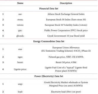
Table 1 summarizes and groups financial data set and energy commodities

data set.

We have to mention here that for the purposes of this paper, we have included EUA into the group of Energy commodity assets, although there are arguments about this like the work of Kanamura (2010) [32] who argue that EUA is not a real commodity asset as those considered in the financial theory.

4. Financial and Econometric Methodology

4.1. Using a VAR Modelling the Conditional Mean

The equation or model of the Conditional mean or first moment is to detect and eliminate any serial correlation in the returns of price data. For a sequence

[image:18.595.212.530.448.688.2]

[image:19.595.207.540.101.420.2]

DOI: 10.4236/jmf.2017.74055 1008 Journal of Mathematical Finance Table 1. The data sets containing the variables employed in the DDC analysis (10-Sep-2007 to 07-Mar-2014).

Name Description

Financial Data Set

1 ase: Athens Stock Exchange General Index 2 stoxx: European Stock 50 Index (Euro stoxx 50) 3 vstoxx: European Stock 50 Volatility Index (vstoxx) 4 ppc: Public Power Corporation (PPC) Stock price 5 gbonds: Greek Government 10 year Bond yield

Energy Commodities Data Set

1 eua: _{(EU Emissions Trading Scheme): €/tCO}European Union Allowance

2 (Phase II) 2 ngas: Natural gas price, NBP, UK €/MWh 3 brent: Brent Oil price, €/bbl

4 Lignite price: Lignite Fuel Cost of a “typical” Lignite-fired _{Power plant (€/MWh)}

Power (Electricity) Data Set

1 smp: Greek Electricity Market wholesale or System _{Marginal Price (ex-ante) (€/MWh)}

2 load: Electricity load (Mw) (ex-post)

of random variables

{ }

Xt the conditional mean (or conditional expectation),

given its past values is defined as: E X X t−1,Xt−2,,Xt j− . As we will see in

Section 5.1, by applying the Ljung-Box test statistics, there is strong evidence of significant serial correlation in the returns. Vector Autoregression (VAR) of lag order p is used in this paper to estimate the first moment.

Let rt symbolizes a k×1 vector of returns at time t, rt =

{ }

ri t, , where ri t, is the daily log returns, for i=1,,k. The VAR(p) model is written as

0 1

0 1 1

or

p

t j t j t

j

t t p t p t

− =

− −

= + +

= + + + +

∑

r r

r r  r

Φ Φ

Φ Φ Φ

ε

ε (5)

where Φ0 is a k×1 vector of constants, Φj k×k matrix of coefficients and

t

ε

_a k×1 vector of residuals. The “optimum” lag length p of the VAR(p) can be found by minimizing the Akaike Information Criterion (AIC). The specifi-cation then of the “best” model, based on AIC, is accepted if the residual “pass” successfully a number of diagnostic tests (e.g. checking for remaining serial cor-relation).

As an example, let k=3, a trivariate model r=

(

ase stoxx vstoxx, ,

)

′ and let 2

DOI: 10.4236/jmf.2017.74055 1009 Journal of Mathematical Finance 1,0 11,1 12,1 13,1

2,0 21,1 22,1 23,1

3,0 31,1 32,1 33,1

11,2 12,2 13,2

21,2 22,2 23,2

31,2 32,2 33,2

, , 1

, , 1

, , 1

ase t ase t

stoxx t stoxx t

vstoxx t vstoxx t

Φ  Φ Φ Φ  −

   

   

 _{= Φ + Φ Φ Φ ⋅} ₋ 

   

   

    −

  Φ Φ Φ Φ  

  _{   }  

Φ Φ Φ 

 

+ Φ_ Φ Φ

Φ Φ Φ

  , , , , 2 , 2 , 2 ase t stoxx t vstoxx t ase t stoxx t vstoxx t ε ε ε   −       ⋅ − +  _{ }     − _{ } _

Serially uncorrelated residuals are generated by a well-specified model for the first moment of the returns. However, heteroskedasticity (the time-varying va-riance of the residuals) will remain in the returns, as it is frequently the case in Energy and financial markets. This feature and the excess kurtosis in the returns call for the GARCH-type estimation approach (Engle, 1982 [40], Bollerslev, 1986 [41]). The GARCH model incorporates the heteroskedasticity characteristic of the data. The works of Chevallier et al. (2009) [10], Benz and Truck (2009) [42], Mansanet-Bataller and Soriano (2009) [6] refer to the application of this type of model in Carbon (EUA) and energy market time series.

Let that the mean of a return time series follows an autoregressive of order p, AR(p), specification

, , ,

1 p

i t o j i t j i t

j

r a a r − ε

=

= +

∑

+ ₍₆₎

where ri t, is the daily log returns of K time series for i=1,,K, εi t, is the residual of series i and ao the drift term.

Suppose that Ft−1 is the set of all available information about the process, up to the time t−1, then the conditional variance of the residual εi t, is

2 ,

i t

σ _{, so}

(

2

)

, 1~ 0, ,

i t Ft N i t

ε ₋ σ _or ε_{i t,} =σ_{i t,}n_t where n_t~NID

( )

0,1 .

This εi t, residual is fitted in the GARCH-type models, described below, to capture the dynamics of the conditional variance.

Let the evolution of the conditional variance in the generic univariate process for each asset, is written as

[

]

2

1 1 1

Q

P O

p t p o t o t o q t q

p o q

I o

δ δ δ

δ

σ ω α ε₋ γ ε₋ ε₋ β σ₋

= = =

= +

∑

+

∑

< +

∑

₍₇₎

where δ _{is either 1 for threshold ARCH also known as AVGARCH, ZARCH}

(Taylor, 1986 [43], Zakoian, 1994 [44]) or 2 for ARCH, GARCH or GJR-GARCH models (Glosten et al., 1993 [45]). In this paper we consider the case of δ =2 and particularly the case GJR-GARCH(P,O,Q). In fact, we fit our data in a GJR-GARCH(1,1,1) model, the dynamics of which is written as

[ 1 ]

2 2 2 2

1 1 1 1 _t 0 1 1

t t t Iε t

σ

= +

ω α ε

− +

γ ε

− ₋< +

β σ

− (8)

where I[εt−1<0] is an indicator function that takes the value 1 if

ε

t−1<0 and 0

DOI: 10.4236/jmf.2017.74055 1010 Journal of Mathematical Finance stationary, 1 1 1

1

1 2

α + γ +β < _{(mean reverting model). In case}

α β

₁+ ₁=1 we

have an integrated model.

In estimating hit from univariate volatility models, the BIC Schwartz Infor-mation Criterion is use to select suitable candidate models that capture the sty-lized facts of the asset return.

4.2. Constant Conditional Correlation (CCC) and Dynamic

Conditional Correlation, DCC, Models

A multivariate GARCH(P,O,Q) is a natural extension of the univariate model, and allows for the time-varying correlations between two series, in addition to their conditional variances. To generate a vector of residuals (hopefully serially uncorrelated) we could use a Vector Autoregression model, VAR(p), to model the mean of a 11 × _{1 vector consisting of the members of the financial, energy}

and power group of data set, given in Table 1. The model produces the follow-ing vector of residuals

(

,, ,, ,, ,, ,, ,, ,, ,, ,,, ,, ,,

)

t

ε

ase t

ε

stoxx t

ε

vstoxx t

ε

ppc t

ε

gbonds t

ε

eua t

ε

ngas t

ε

brent t

ε

smp t

ε

lignite t

ε

load t

′ =

ε

We also suppose that the underlying distribution of returns follows a condi-tional multivariate normal process, therefore we can write εt Ft−1~N

(

0,Ht

)

,

where Ft−1 is a filtration i.e. an information set about the time series up to the time step t−1. Thus, the

ε

t is conditionally heteroskedastic, which means that

t= Ht⋅nt

ε _{, where} n_t~N

( )

0,I an iid error process.

For modelling Ht a number of specifications has been suggested, the most commonly mentioned is the generic VECH-model, developed by Bollerslev et al. (1986) [41], the CCC-model (Constant Conditional Correlation) also by Bol-lerslev (1990) [46] and the BEKK-model by Engle and Kroner (1995) [2]. A de-tailed survey on multivariate GARCH models is provided by Silvennoinen and Tersvirta (2007) [47].

In this paper will apply the parsimonious Dynamic Conditional Correlation (DCC) approach, developed by Engle (2002) [48] and Engle and Sheppard (2001) [49]. This model is actually a natural extension of the CCC-model, giving the opportunity for a two-stage estimation of the dynamic evolution of condi-tional correlations between, for example, two commodities. In the first stage of the procedure, standardized residuals are generated by univariate GARCH mod-els fitted on the data of the individual time series. In the second stage the corre-lation process is estimated.

According to the work of Engle and Sheppard (2001) [49], the conditional covariance matrix Ht is written as follows

t t t t

H =D R D (9)

where Dt a k×k diagonal matrix with elements 2

, i t

σ

_{on the ith diagonal}

DOI: 10.4236/jmf.2017.74055 1011 Journal of Mathematical Finance t

R is the time-varying conditional correlation matrix. In the case of

CCC-model we have:

Model 1: Ht=D RDt t (10)

( )

ij

R= ρ

where R = Constant Conditional Correlation. The assumption that conditional correlations are constant is unrealistic in particular applications, although the estimation of CCC parameters is simpler. We use CCC hare as a benchmark for testing the consistency of correlations (see Table 6 below).

The log-likelihood is our case, for the vector θ _{of parameters is given by}

( )

(

( )

( )

( )

1

)

1

1 _{log 2π}

2 log log 2

T

t t t t

t

t

L θ m D R R−

=

′

= −

∑

+ + +ξ ξ ₍₁₁₎

where ξ_t ~N

(

0,R_t

)

the standardized residuals, t t t

D

=ε ξ _.

In case that the conditional distribution of

ε

t is not normal, Equation (9) is the Quasi-likelihood function. The dynamic correlation specification suggested by Engle and Sheppard (2001) [49] is:

(

)

1 1 1 1

1

Q Q

P P

t j j j t j t j j t j

j j j j

Q α β Q α _{− −} β Q₋

= = = =

 

′

= −_ − _ + +



∑

∑



∑

ξ ξ

∑

(12)

where Q is the k×k unconditional covariance matrix of the standardized

residuals, generated from the first stage of the process. The extent to which

ξ

t affect the dynamics of the correlation is captured by the αj, while βj is a

pa-rameter measuring the decay in dynamics. If we plug α_j =β_j=0 into (11), the

CCC model of Bollerslev (1990) [46] is obtained. The lag-lengths of residuals and decay are expressed by P and Q (not to be confused with those in Equa-tion (6)). Finally, the dynamic condiEqua-tional correlaEqua-tion is written

* 1 * 1

t t t t

R =Q Q Q− − (13)

where *

t

Q is a diagonal matrix (k×k) consisting of the square root of the

di-agonal elements of Qt. Furthermore, the conditional covariance matrix Rt of the residuals generated by VAR(p), is obtained by standardizing these residuals by the conditional variances, so a typical element of Rt is

, , , ,

, , , ,

i j t i j t

i i t j j t

q

q q

ρ = (14)

In the framework of this paper estimation, the indices range as , , , , , , , , , ,

i j=ase stoxx vstoxx ppc eua ngas brent smp load lignite

By letting P= =Q 1 in Equation (11) we obtained our DCC model 2 speci-fication:

DOI: 10.4236/jmf.2017.74055 1012 Journal of Mathematical Finance [50], typical values of the dynamic parameters α α β, + are α β+ >0.80 and

0.04

α ≤ _{while in financial application, in particular,} α β+ ≥0.96 and 0.04

α ≤ _. Q=E

[ ]

ξ_tξ_t′ is the unconditional correlation (the unconditional va-riance matrix of the standardize residuals. A typical element of the correlation matrix Rt, regarding the interaction, for example, between ase index and ppc stock price is

, , , ,

, , , ,

ase ppc t ase ppc t

ase ppc t ase ppc t

q

q q

ρ = (16)

Therefore, by using model 2 above, we have

(

)

(

)

, , 1 , , 1 , 1 , , 1

ase ppc t ase ppc ase t ppc t ase ppc t

q = − −α β q +α ξ −ξ′ − +βq − (17)

(

)

(

2

)

, 1 , 1 , 1

ase t ase ase t ase t

q = − −α β q +α ξ − +βq − (18)

(

)

(

2

)

, 1 , 1 , 1

ppc t ppc ppc t ppc t

q = − −α β q +α ξ − +βq − (19)

Model 1 will be our basic reference model. This scalar DCC specification is the most parsimonious one because of the assumption that all commodities correla-tions “obey” the same ARMA(P,Q) type specification, which means that they are all governed by the same coefficients

α

_and

β

. The above assumption might be a valid one, in the case of similar commodities (or “assets” in general), be-longing in same asset category or class. However, in our case, our “assets” belong to different categories, namely financial, energy and power; therefore it is a rea-sonable assumption that these markets exhibit “asset” specific correlation sensi-tivities. To face this dissimilarity in asset’s class, a generalization of the DCC model has been suggested, incorporating also the impact of any asymmetries on the correlation dynamics. It is known that in a Markov Switching Model (MSM) or in a Threshold Autoregressive Model (TARM), the conditional correlations are allowed to have different evolutionary dynamics. Instead this is not the case for DCC model in which the correlations follow the same dynamics. This is a li-mitation of the DCC. For example, if the data exhibit structural breaks, DCC model can give misleading conclusions. Another limitation of DCC is that it does not work reliably for large number of assets. Cappielo et al. (2006) [51] have developed a number of various asymmetric multivariate GARCH models to capture the asymmetries. For an in depth description of the “mathematical” properties, its limitation and inconsistencies in DCC model, Aielli (2011) [50] provides an excellent work.

4.3. The Asymmetric Generalized DCC Model

Engle (2002) [48] propose a Generalized Dynamic Conditional Correlation (G-DCC) in order to tackle the correlation across asset categories, a flexible model allowing for asset specific correlation parameters. The model is written as

DOI: 10.4236/jmf.2017.74055 1013 Journal of Mathematical Finance

{ }

ii

B= β .

The positive definiteness requirement is satisfied by

α

_ii+

β

_ii<1 and , 0, ,

ii ii i j

α β

≥ ∀ _{. The above specification tackles the dissimilarity of asset}

prob-lem by allowing for a high degree of dissimilarity in correlations.

The advantage of G-DCC over the simple scalar DCC is that it can generate a variety of correlation patterns. The coefficients

α

ii can be considered for mea-suring the sensitivity of the correlation of asset i with other assets to

correla-tion residuals (Hafner and Frances, 2003) [52]. High values for

α

ii in combi-nation with low values for

β

ii result in almost horizontal, very flat correlations of asset i with any other asset in the specification. Instead, low values for

α

ii combined with high values for

β

ii produce very fluctuating correlations.

Cappielo et al. (2006) [51] proposes a further generalization, the AG-DCC (Asymmetric Generalized DCC) model 4 that actually nests model 4, written as

Model 4: Qt=

(

Q−A′QA−B′QB−G NG′

)

+A′ξ ξt−1 t′−1A+B Q B′ t−1 +G′n nt−1 ′t−1G (21)" where G is a k×k diagonal matrix of parameters, G=

{ }

g_ii ,n_t=

{ }

n_{i t,} a

1

k× vector with n_{i t,} =min

(

ξ_t, 0

)

, N is a k×k matrix of constants,

1 1 t T

t t

T

N= −

∑

₌n n′.

Similarly as in model 3, the positive definiteness requirement is satisfied by 1

ii ii n ki

α

+

β

+ < _and

α β

_ii, _ii,n_i≥0, for i=1,,k where k is the maximum

eigenvalue of Q N Q (Cappielo et al., 2006) [51].

Model 4 is further extended to include control (“exogenous”) variables Vargas (2008) [53] proposed the AG-DCC-X model and it is this model used by Koen-ing (2011) [20] to test the hypothesis of the effect of static merit order regimes on correlation between input fuels, carbon emission and electricity prices. We do not consider the model in this paper but we have included for the complete-ness of our review.

By using that _A′_{∗ =A A B}2_, ′_{∗ =B B}2 etc., little algebra transforms model 3 into the following form

(

2 2

)

2 2 2

(

)

1 1 1 1 1

1

t t t t t t

Q = −A −B Q+Aξ ξ− ′− +B Q− +G n n− ′− −N (22)

5. Empirical Findings

5.1 Data Tests and Applied Methodology

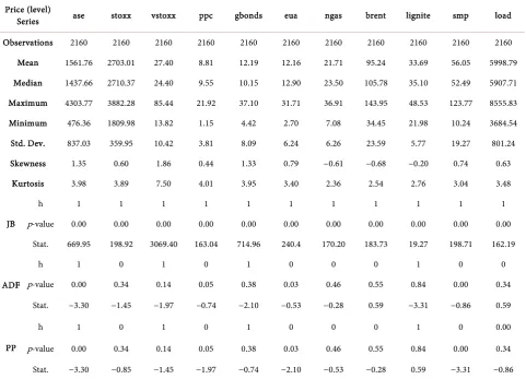
In this subsection we present the empirical findings, while in Section 5.2 we comment on these findings in details. Table 2 provides the summary statistics of price levels and of the electricity load (demand). The correlation matrix of all variables (raw data) is shown in Table 3. While Table 4 provides summary sta-tistics of log returns of the variables considered.

[image:25.595.58.540.91.438.2]

DOI: 10.4236/jmf.2017.74055 1014 Journal of Mathematical Finance Table 2. Summary statistics of price (levels) (8-Apr-2008 to 07-Mar-2014).

Price (level)

Series ase stoxx vstoxx ppc gbonds eua ngas brent lignite smp load

Observations 2160 2160 2160 2160 2160 2160 2160 2160 2160 2160 2160 Mean 1561.76 2703.01 27.40 8.81 12.19 12.16 21.71 95.24 33.69 56.05 5998.79 Median 1437.66 2710.37 24.40 9.55 10.15 12.90 23.50 105.78 35.10 52.49 5907.71 Maximum 4303.77 3882.28 85.44 21.92 37.10 31.71 36.91 143.95 48.53 123.77 8555.83 Minimum 476.36 1809.98 13.82 1.15 4.42 2.70 7.08 34.45 21.98 10.24 3684.54 Std. Dev. 837.03 359.95 10.42 3.81 8.09 6.24 6.26 23.59 5.77 19.27 801.24 Skewness 1.35 0.60 1.86 0.44 1.33 0.79 −0.61 −0.68 −0.20 0.74 0.63

Kurtosis 3.98 3.89 7.50 4.01 3.95 3.40 2.36 2.54 2.76 3.04 3.48

JB

h 1 1 1 1 1 1 1 1 1 1 1

p-value 0.00 0.00 0.00 0.00 0.00 0.00 0.00 0.00 0.00 0.00 0.00 Stat. 669.95 198.92 3069.40 163.04 714.96 240.4 170.20 183.73 19.27 198.71 162.19

ADF

h 1 0 1 0 1 0 0 0 1 0 0

p-value 0.00 0.34 0.14 0.05 0.38 0.03 0.46 0.55 0.84 0.00 0.34

Stat. −3.30 −1.45 −1.97 −0.74 −2.10 −0.53 −0.28 0.59 −3.31 −0.86 0.59

PP

h 1 0 1 0 1 0 0 0 1 0 0.00

p-value 0.00 0.34 0.14 0.05 0.38 0.03 0.46 0.55 0.84 0.00 0.34

Stat. −3.30 −0.85 −1.45 −1.97 −0.74 −2.10 −0.53 −0.28 0.59 −3.31 −0.86

Interpretation of the Boolean variable h: h = 1 the null hypothesis of the test is rejected, h = 0 fail to reject the null hypothesis of the test. JB test the null hypothesis of normality, ADF and PP test the null hypothesis of unit root.

Table 3. Correlation matrix between levels of variables considered in this study.

“ase” “stoxx” “vstoxx” “ppc” “gbonds” “eua” “ngUK” “brent” “lignite” “smp” “load”

“ase” 1 0.6504 0.0851 0.8790 −0.6797 0.8527 −0.2440 −0.2276 −0.7683 0.2562 0.3134

“stoxx” - 1 −0.5302 0.7323 −0.4838 0.4718 0.2077 0.3467 −0.1803 0.1619 0.0633

“vstoxx” - - 1 −0.0913 −0.0307 0.2897 −0.1447 −0.5587 −0.4267 0.3028 0.1319

“ppc” - - - 1 −0.7478 0.7086 −0.2340 −0.1821 −0.4764 0.1143 0.2468 “gbonds” - - - - 1 −0.4271 0.2796 0.4740 0.3777 0.1455 −0.0716

“eua” - - - 1 −0.1364 −0.1550 −0.8159 0.4379 0.4122 “ngUK” - - - 1 0.6567 0.2481 0.3734 −0.1327 “brent” - - - 1 0.3749 0.1706 −0.0773 “lignite” - - - 1 −0.3414 −0.3944

“smp” - - - 1 0.4675

[image:25.595.56.544.496.737.2]

[image:26.595.55.540.90.609.2]

DOI: 10.4236/jmf.2017.74055 1015 Journal of Mathematical Finance Table 4. Daily log returns summary statistics (08-Apr-2007 to 07-Mar-2014).

Log Return Series ase stoxx vstoxx ppc gbonds eua ngas brent lignite smp load Panel A: Descriptive statistics

Observations 2159 2159 2159 2159 2159 2159 2159 2159 2159 2159 2159 Mean 0.00 0.00 0.00 0.00 0.00 0.00 0.00 0.00 0.00 0.00 0.00

Median 0 0 0 0 0 0 0 0 0 0 0

Maximum 0.13 0.10 0.33 0.22 0.14 0.24 0.36 0.18 0.29 1.02 0.20 Minimum −0.10 −0.08 −0.27 −0.25 −0.68 −0.43 −0.11 −0.17 −0.25 −0.87 −0.25

Std. Dev. 0.02 0.01 0.05 0.03 0.02 0.03 0.02 0.02 0.02 0.16 0.04 Skewness 0.06 0.12 0.86 −0.18 −12.55 −1.21 3.29 0.02 4.21 0.03 −0.63

Kurtosis 7.31 11.32 8.09 10.70 327.73 34.44 46.55 16.49 103.69 8.82 10.22

JB (p-value)

h 1 1 1 1 1 1 1 1 1 1 1.00

p-value 0.00 0.00 0.00 0.00 0.00 0.00 0.00 0.00 0.00 0.00 0.00 Stat. 1670 6231.9 2591.4 5342.8 9543009.1 89462.8 174476.26 16361.3 918408.54 3051.87 4831.9 Panel B: Stationarity

ADF

h1 1 1 1 1 1 1 1 1 1 1 1

p-value 0.000 0.000 0.000 0.00 0.00 0.00 0.00 0.00 0.00 0.00 0.00 Stat. −43.78 −45.64 −46.43 −42.92 −42.06 −44.7 −47.17 −58.80 −62.95 −52.21 −58.80

PP

h 1 1 1 1 1 1 1 1 1 1 0.00

p-value 0.000 0.00 0.00 0.00 0.00 0.00 0.00 0.00 0.00 0.00 0.00 Stat. −43.78 −45.64 −46.43 −42.92 −42.06 −44.7 −46.43 −47.17 −58.80 −62.95 −52.21 Panel C: Serial Correlation. ARCH tests

Q (20)

h 0 1 1 1 1 1 1 1 1 1 1

p-value 0.06 0.00 0.00 0.00 0.00 0.00 0.00 0.00 0.00 0.00 0.00 Stat. 30.7 56.53 52.55 52.41 58.22 67.50 53.44 41.76 187.97 243.84 162.24

Q2 ₍₂₀₎

h 1 1 1 1 0 1 0 1 1 1 1

p-value 0. 0.00 0.00 0.00 0.99 0.00 0.94 0.00 0.00 0.00 0.00 Stat. 250.8 888.27 166.38 280.2 1.18 154.9 11.06 386.1 286.8 376.23 125.35

ARCH-L M (20)

h 1 1 1 1 0 1 0 1 1 1 1

p-value 0.000 0.00 0.00 0.00 0.99 0.00 0.98 0.00 0.00 0.00 0.00 Stat. 155.45 408.07 119.35 182.30 1.13 120 9.42 206.8 247.3 240.01 120.82

Q (20) and Q2 _{(20) are Ljung-Box or Q statistics for testing the null hypothesis of no autocorrelation in the residuals. The 5% critical values of X}2 ₍₂₀₎

dis-tributions is 31.41. For ADF and PP test, the 1% critical value is −3.44.

DOI: 10.4236/jmf.2017.74055 1016 Journal of Mathematical Finance we present the results of the dynamic conditional correlation. Also, the uncondi-tional correlation between electricity market (smp) and EUA market (eua) was found as expected, positive (0.4376) indicating that there is connection between the price of CO2 quotas and SMP. However the DCC between them is much smaller, as it will be described later on.

By observing Table 4 we conclude that financial, energy and electricity “asset” returns are likely to be non-Gaussian. In all returns the skewness is non-zero, an evidence of a non-symmetric distribution. Furthermore, the kurtosis is signifi-cantly in excess (>3) which indicates fat tails of the distribution, containing more probability than a normal distribution. In combination, the log returns of “as-sets” are leptokurtic. Also, we test the return for normality by applying the Jar-que-Bera (JB) test statistic. According to this test the joint null hypothesis is that both skewness and excess kurtosis are zero. As we observe in Table 4, the

p-value for the JB statistics is zero in all returns, therefore the null hypothesis can safely be rejected, so the returns follow a non-normal distribution.

We have also applied the Augmented-Dickey-Fuller (ADF) and Phil-lips-Perron (PP) unit root tests. As we observe, both tests give values larger than the critical value for the 1% level of significance. Therefore, we can reject the null-hypothesis of a unit root for all returns, so they are taken to be statio-nary.

To detect autocorrelations in the returns we have used the Ljung-Box or Q statistic. From Table 4 also, we see that all returns show signs of statistically significant autocorrelation (gbonds’ and ngas’ statistics are less than 31.41, but with p-values of 0.99 and 0.94 respectively). The strongest autocorrelation is in smp, lignite and load returns (with Q(20) statistics 243.84, 187.97 and 162.24 respectively).

All log returns have a mean zero. GEM wholesale price (smp) returns are most volatile (std. Dev  0.16) followed by vstoxx and load returns, while stoxx returns are the less volatile.

All returns show evidence of volatility clustering (ARCH effects) as the visual inspection of the log return (see Figures 9-11) and the ARCH-Lagrangean Multiplier (ARCH-LM) test in Table 4 show, as the test statistic is significantly higher than its critical value for the 5% significance. The gbonds and ngas re-turns’ test stat is below the critical value, however the corresponding p-values are extremely high (0.99 and 0.98 respectively), so we cannot refuse the existence of ARCH effects.

Figures 9-11 depict the dynamic evolution of the returns of the time series

DOI: 10.4236/jmf.2017.74055 1017 Journal of Mathematical Finance Figure 9. Log-returns of the financial set’s time series for the period 10-Sep-2007 to 07-Mar-2014.

Figure 10. Log-returns of the energy (commodity) data set’s time series for the period 10-Sep-2007 to 07-Mar-2014.

returns exhibiting volatility clustering. The ARCH-LM test results, mentioned before, confirm the existence of this stylized fact.

[image:28.595.216.534.70.301.2] [image:28.595.213.536.346.590.2]

[image:29.595.215.531.84.332.2]

DOI: 10.4236/jmf.2017.74055 1018 Journal of Mathematical Finance Figure 11. Log-returns of the electricity data set’s time series for the period 10-Sep-2007 to 07-Mar-2014.

the fitted GARCH(1,1) model on each individual asset are given in Table 5. Af-ter we obtain the residuals from the mean equation we proceed by estimating the DCC between the assets. Table 6 shows the estimation for the DCC-GARCH (1,1) model. The coefficients α and β for