Contribution to Development of Reliability and
Optimization Methods Applied to Mechanical
Structures
Siham Ouhimmou1, Abdelkhalak El Hami2, Rachid Ellaia3, Mohamed Tkiouat3 1
Laboratory of Mechanics, University Hassan II, Casablanca, Morocco 2
Laboratory of Mechanics of Rouen, National Institute of Applied Sciences, Rouen, France 3
Laboratory of Study and Research in Mathematics Applied, Mohammedia School of Engineers, Agdal-Rabat, Morocco
Email: [email protected], [email protected]
Received June 11, 2012; revised November 8, 2012; accepted November 15, 2012
ABSTRACT
In order to take into account the uncertainties linked to the variables in the evaluation of the statistical properties of structural response, a reliability approach with probabilistic aspect was considered. This is called the Probabilistic Transformation Method (PTM). This method is readily applicable when the function between the input and the output of the system is explicit. However, the situation is much more involved when it is necessary to perform the evaluation of implicit function between the input and the output of the system through numerical models. In this work, we propose a technique that combines Finite Element Analysis (FEA) and Probabilistic Transformation Method (PTM) to evaluate the Probability Density Function (PDF) of response where the function between the input and the output of the system is implicit. This technique is based on the numerical simulations of the Finite Element Analysis (FEA) and the Prob- abilistic Transformation Method (PTM) using an interface between Finite Element software and Matlab. Some prob- lems of structures are treated in order to prove the applicability of the proposed technique. Moreover, the obtained re- sults are compared to those obtained by the reference method of Monte Carlo. A second aim of this work is to develop an algorithm of global optimization using the local method SQP, because of its effectiveness and its rapidity of conver- gence. For this reason, we have combined the method SQP with the Multi start method. This developed algorithm is tested on test functions comparing with other methods such as the method of Particle Swarm Optimization (PSO). In order to test the applicability of the proposed approach, a structure is optimized under reliability constraints.
Keywords: Reliability Methods; Probabilistic Transformation Method; Finite Element Analysis; FEACPTM; The Method SQP; The Multi Start Method; Algorithm MSQP; Structural Optimization
1. Introduction
As the properties of the realistic structure, the model is necessary to take into account some uncertainty. This un- certainty can be conveniently described in terms of pro- bability measures, such as distribution functions. It is a major goal of reliability methods to relate the uncertain-ties of the input variables to the uncertainty of the struc-tural performance. A fundamental problem in strucstruc-tural reliability analysis is the computation of the probability integral ([1-5]):
0 0
f
G X
P Prob G X f X X
d
(1)
where in which is the transpose, is a vector of random variables representing the uncertain parameters of considered structure,
T1, , n
X X X T
f X is the prob-
ability density function of X, is the Limit State Function defined such that: is the domain of integration denoted the failure set, and
G X
0 G X f
P is the prob- ability of failure. The difficulty of computing this inte- gration led to development of various methods of reli- ability analysis such as Monte Carlo, FORM and SORM ([6-8]), and Probabilistic Transformation Method PTM.
Method PTM program; and 4) concluding the probability of failure and reliability of systems. To show the advan- tage of the proposed method, we have carried out diffe- rent applications to cover several structural problems.
2. Reliability Method of Analysis
2.1. Finite Element Analysis
The finite element method is the standard tool for certain classes of partial differential equations arising in various fields of engineering and in particular for those arising in solid mechanics. For linear systems enforcing global sta- tic or dynamic equilibrium, the FE method leads to a sys- tem of linear equations, respectively
KU F (1)
MU t CU t KU t F t (2) where the matrix K is the global stiffness matrix, M
is the mass matrix, U the vector of displacement, F
the vector of applied loads, C is the damping matrix. These matrix obtained by adding the contributions of all element matrix. There are symmetrical and positive vectors.
e e
K
K (3)e e
M
M (4) The latter matrix has the form,d
e
e e e
K D B
ee
(5)
d
e
e e eT e
M H H
(6)where is the matrix relating element displacements and strains, is the elasticity matrix relating stresses and strains,
e B
e D
e
is the mass density, He
is the shape functions and is the spatial domain of the element. The global damping matrix C is typically formulated in terms of M and K.
e
2.2. Probabilistic Transformation Method PTM
The Probabilistic Transformation Method is based on the following theorem:
Theorem: Suppose that X is a continuous random
variable with PDF f x
and is the one-di- mensional space where , is differentiable and monotonic. Consider the random variableA 0
f x
Y u X , where yu x
defines a one-to-one transformation that maps the set A onto a set B so that the equation
yu x can be uniquely solved for x in terms of , say
y
1
xu y . Then, the PDF of Y is
1
Y X
f Y f u y J (7)
where,
1
d d
d d
u y
x J
y y
is the Jacobean transforma-
tion, which must be continuous for all points yB. The PTM is based on one-to-one mapping between the random output(s) and input(s) where the transformation J. Jacobean can be computed. The PDF of the output(s) is then computed through the known joint PDF of the in- puts multiplied by the determinant of the Jacobean ma- trix.
The idea of PTM is based on the following formula [9]:
u z
f u J f z (8)
z J
u
(9)
u
f u is the probability density function of the variable
u.
z
f z is the probability density function of the variable
z.
The Probabilistic Transformation Method (PTM) is one of the most widely used methods in reliability analy- sis. However, this method has drawbacks in the solution of reliability problems. It requires the evaluation of the explicit response functions with respect to the random variables that is very difficult in analysis of complicated structures. To overcome these drawbacks, an interface between the Finite Element Analysis and The Probabilis- tic Transformation Method (PTM) is proposed in this pa- per.
2.3. Finite Element Analysis Coupled with Probabilistic Transformation Method: FEACPTM
The Finite Element Analysis (FEA) software is used to perform the structural analysis to obtain the maximal dis- placement of the structure, and maximal stress, corrs- ponding to a set of given design variables ([10-12]). These analysis results are sent to the reliability program to conduct the Probabilistic Density Function PDF, and the probability of failure and generate new random vari- ables. The newly generated variables are then used to update the input file. The Finite Element Analysis (FEA) software is then invoked again to perform the structural analysis with the new input parameters. This process is repeated until satisfactory results are obtained.
2.3.1. Interface between FEA Software and Reliability Analysis Program
type of implementation, the FEA is viewed as a black box in the analysis process and the FE code is communi- cated with through a generic interface, through the input files of the latter. The reliability analysis program con- trols the FE code by automatically modifying the input files, set identifiers, which govern the automatic genera- tion of input file samples by the stochastic solver, using pattern matching and replacement.
2.3.2. Algorithm of Method FEACPTM
The outline of a Proposed Method FEACPTM is as fol- lows:
1) Generate the input random variables;
2) Calculate the value of output variables by FE soft- ware. For each value of input the correspondent value of output is estimating using FEA and stocking it in solu- tion file;
3) Approximate the function between input and output variables using Spline Interpolation;
4) Calculate of the determinant of Jacobean of input and output variables (Equation (9));
5) Apply the basic relation of PTM (Equation (8)); 6) Evaluate the graphic of PDF of output variable in function of this output variables (in our case the PDF of displacement in function of displacement);
7) Approximate the Probability of failure Pf. 2.4. Application
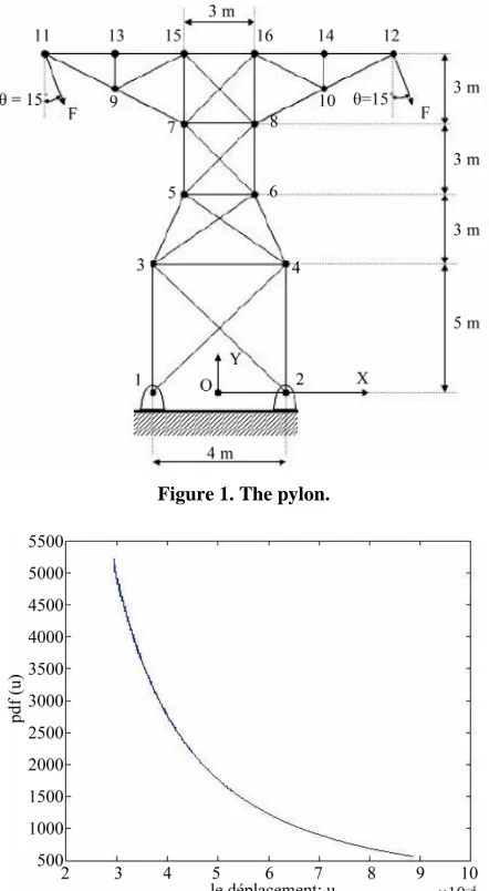
We are going to analyze the reliability of the pylon of a line of transportation of electricity that one assimilates to a truss plan. Two identical loads F of 1.8 KN are applied to the two superior extremities of the following pylon an angle of 15. The bars forming the pylon are in steel of which Young’s modulus E = [100 GPa, 300 GPa] and the Poisson coefficient 0.29. The section of every bar is worth A = 27.90 cm2. The hypothesis for this prob- lem is that the weight of each bar of the pylon is negligi- ble in front of the applied efforts (see Figure 1).
This structure is analyzed using the FEA software for structural modelling, and static analysis in which the FEA software is used to approximate the structural re- sponse, this response is used by the PTM program for computing the probability of failure. For that purpose, statistic models must be defined for each random vari- able involved. In this case, the Young’s modulus E is uniformly distributed in the range [100 GPa, 300 GPa]. Using the proposed technique FEACPTM, we obtain the following graph (see Figure 2):
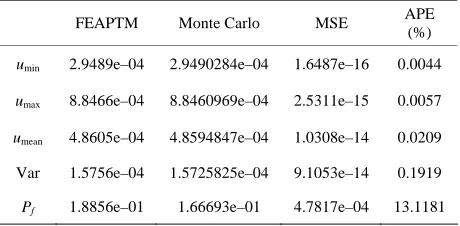
The PDFs of the normalized vertical displacement uy
are plotted in Figure 2 assuming that the variable uy is
[image:3.595.313.534.85.487.2]independent and uniformly distributed in the range [2.9489e04, 8.8466e04]. Also in this case the results are accurate as shown by favourable comparison with clas- sical Monte Carlo simulation. Let us suppose the limit
Figure 1. The pylon.
Figure 2. PDF (u) when E is uniformly distributed.
displacement is u = 6.635e04 mm. It is required to find the failure probability Pf P u
ulimit
Mean Squared Error (MSE) and Absolute Percentage Error (APE) are calculated by using the following equa- tion
2 1 mcMSE u u
(28)
1
100 mc mc u u APE
u
(29)
where 1 the value of displacement obtained with
FEACPTM is, is the predicted value with Monte Carlo simulation.
u
mc u
The numerical values of probabilistic characteristics of the displacement of this pylon are listed in this table.
Table 1. Results obtained by FEACPTM and Monte Carlo si- mulation.
FEAPTM Monte Carlo MSE APE
(%)
umin 2.9489e–04 2.9490284e–04 1.6487e–16 0.0044
umax 8.8466e–04 8.8460969e–04 2.5311e–15 0.0057
umean 4.8605e–04 4.8594847e–04 1.0308e–14 0.0209
Var 1.5756e–04 1.5725825e–04 9.1053e–14 0.1919
Pf 1.8856e–01 1.66693e–01 4.7817e–04 13.1181
since a number of 800 (less than 1000) iterations suffice to obtain results close to those obtained by Monte Carlo simulation. To compare the results, the MSE and APE are calculated. The values of MSE and APE are very small, which shows the accuracy and efficiency of FE- ACPTM.
3. Optimization Method of Analysis
3.1. Sequential Quadratic Programming (SQP) Method
We present Sequential Quadratic Programming (SQP) method for optimization problems involving general lin- ear and nonlinear constraints. This method has proved highly effective for many such problems. It typically finds a (local) optimum from an arbitrary starting point, and they require relatively few evaluations of the prob- lem functions and gradients. The method SQP consist in to resolve an optimization problem for a limited number of variables under the following general form ([13,14]):
Minimize , Subject to 0
0
f X X
h X
g X
(10)
where f X
is the objective function, X is the vector of independents variables of optimization and h X
is the equality constraints, g X
are called “inequality constraints”. An SQP method obtains search directions from a sequence of (Quadratic Problem: QP) sub-prob- lems. Each QP sub-problem minimizes a quadratic model of a certain lagrangian function subject to linearized con- straints. Some merit function is reduced along each search direction to ensure convergence from any starting point.
Minimize , 1 min
2
Subject to 0 0
0
T T
q i i
T
i i
T
i i
f X X
d d H d f X d
h X g X d g X
g X h X d h X
At each iterate a QP sub problem is used to gene- rate a search direction towards the next iterate
i
d Xi1
1
i i i
X X d (12) where the value of i is determinate in each iteration
using one-dimensional minimization method.
i
3.2. Multi Start Algorithm
The multi start method for global optimization can over- come some of the limitations of the local Solving method. This method will automatically run the local method from a number of starting points and will display the best of several locally optimal solutions found, as the prob- able global optimal solution. The multi start algorithm attempts to find a global solution by starting a local solver from multiple starting points in the space of re- search S. This method generates uniformly distributed points in S, and starts local solver from each of these. This converges to a global solution.
3.3. Proposed Algorithm: MSQP
The MSQP Algorithm is a global optimization algorithm; this algorithm is the result of the combination of Multi start algorithm and the SQP method. It resumes the prin- cipal mechanisms of the SQP method to which are added other mechanisms destined to treat multi-modales prob- lems. The solutions found by the SQP method during the execution of each iteration are improved, so that always we keeps the global solution and the local solution is ignored. Thus, at the end of the treatment, we obtain the global solution, that is the solution of the problem mul- timodal. In MSQP algorithm, the aspect of the global search of start Multi algorithm is used to maintain the diversity. In fact, we considering that MSQP algorithm will converge after a small number of iterations to a local solution if we find another local solution, we can con-sider that it is not useful to continue the search from this moment, and it is better to start a new search.
3.4. Results
In order to evaluate the performance of the method pro- posed, we compare the solutions obtained by the MSQP algorithm with the solutions reported in (pPSA: per- turbed Particle Swarm Algorithm and pPSA best [15] for certain functions tests. Table 2 presents different solu- tions obtained by algorithms pPSA, pPSA best and pro- posed algorithm MSQP (see Table 2).
0
(11)
The computational results of MSQP algorithm and the algorithms PSO and TRIBES (that are cited in [16]), are summarized in tables for each example problem. The different results are obtained for a dimension D = 10 for every function test (see Table 3).
Table 2. The solutions obtained by pPSA, pPSA best and MSQP.
Functions npart pPSA pPSA
b t MSQP
2 65.96e– 64.39e– 154.3216e– Sphere
20 66.12e– 64.7e– 157.1525e–
2 41.47e+ 68.06e– 177.3985e– Quadratique
20 53.56e– 69.04e– 83.5531e–
2 21.78e+ 18.76e+ 0.9950 Rastrigin
20 85.9 54.7 7.9597
2 11.83e+ 11.64e+ 75.6056e– Ackley
[image:5.595.57.289.110.229.2]20 17.59e– 31.59e– 51.6215e–
Table 3. The solutions obtained by MSQP, TRIBES and PSO.
Function PSO TRIBES MSQP
Rastrigin 4.02 (100000) 8.5 (100000) 2.9849 (100000)
Rosenbrock 1.88 (100000) 0.06 (1500000) 0.7698 (100000)
Ackley 20.11 (100000) 20.32 (100000) 17.0918 (100000)
proposed MSQP technique was tested on a number of benchmark multimodal mathematical functions and the performance compared with other Global Optimization approaches. The results finding by MSQP algorithm are the best ones for the most functions test.
3.5. Structural Optimization under Reliability Constraints
[image:5.595.351.492.251.406.2]To illustrate the efficacy of the presented algorithm (see
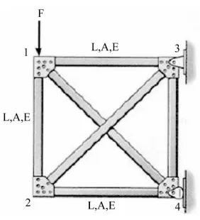
Figure 3) to solve the problems of structural design op-timization under reliability constraint, we choose as ex-ample the truss constituted by six identical bars. For this problem, the objective function to minimize is the section A of each bars of the considered structure; the variables of conception are the dimensions of the section (the height and the width) (see Figure 4).
The geometric and material properties are:
The initial section of every bar A = 0.0015 m2;
The length L = 10 m;
The load F = 10 N;
The Young’s modulus E = 2 × 10⁸ N/ m2.
The minimization of the section is done under con- straints on the design variables and under a reliability constraint (the probability of failure of the structure must not surpass a value limit). The formulation of the opti- mization problem for the section of each bar of truss is the following:
,
min *
Subject to 1 and 5
6.32 6.33
0.22 0.001 *
w t
f
f w t
w t
w t
P w t
(13)
Initialize i1
Until (Stopping condition is not satisfied)
Step 1: (generation) Construction of the solution Xi
For i1 to don Step 2: (research)
Apply SQP algorithm (fmincon) to find Xopt
Let Xopt be the solution obtained If Xopt improves the best solution Update the best
i = i + 1 End For End Until
Figure 3. The basic steps of the MSQP algorithm.
Figure 4. Truss constituted by 6 bars.
where w is the width and t is the height.
To resolve this problem of structural optimization un- der reliability constraint, we used the algorithm MSQP developed in the preceding sections. Therefore, we ob- tained as results of this problem the following values: w = 1.32 cm, t = 5 cm and A = 6.6e–4 m2.
4. Conclusion
[image:5.595.56.289.262.323.2]proved the robustness and high performance. The pro- posed algorithm MSQP is applied to solve structural pro- blems under reliability constraints.
REFERENCES
[1] M. Lemaire, “Evaluation of Reliability Index Associated to Structural Mechanical Models,” French Journal of Mechanic, Vol. 2, 1992, pp. 145-154.
[2] B. Sudreta and A. Der Kiureghian, “Comparison of Finite Element Reliability Methods,” Probabilistic Engineering Mechanics,Vol. 17, No. 4, 2002, pp. 337-348.
doi:10.1016/S0266-8920(02)00031-0
[3] A. Der Kiureghian and J.-B. Ke, “The Stochastic Finite Element Method in Structural Reliability,” Probabilistic Engineering Mechanics, Vol. 3, No. 2, 1988, pp. 83-91.
doi:10.1016/0266-8920(88)90019-7
[4] A. M. Hasofer and N. C. Lind, “Exact and Invariant Se- cond-Moment Code Format,” Journal of the Engineering Mechanics Division, Vol. 100, No. 1, 1974, pp. 111-121.
[5] H. O. Madsen, S. Kenk and N. C. Lind, “Methods of Struc- tural Safety,” Prentice-Hall Inc., Upper Saddle River, 1986.
[6] R. Rackwitz, “Reliability Analysis: A Review and Some Perspectives,” Structural Safety, Vol. 23, No. 4, 2001, pp. 365-395. doi:10.1016/S0167-4730(02)00009-7
[7] M. Lemaire, A. Mohamed and O. Flores-Macias, “The Use of Finite Element Codes for the Reliability of Struc- tural Systems,” 1997.
[8] A. Mohamed and M. Lemaire, “Linearzed Mechanical
Model to Evaluate Reliability off Shore Structures,” Struc- tural Safety, Vol. 17, No. 3, 1995, pp. 167-193.
doi:10.1016/0167-4730(95)00009-S
[9] S. Kadry, “A Proposed Technique to Evaluate the Sto-chastic Mechanical Response Based on Transformation with Finite Element Method,” International Journal of Applied Mathematics and Mechanics, Vol. 2, No. 2, 2006, pp. 94-108.
[10] G. Muscolino, G. Ricciardi and N. Impollonia, “Improved Dynamic Analysis of Structures with Mechanical Uncer-tainties under Deterministic Input,” Structural Safety, Vol. 15, No. 2, 2000, pp. 199-212.
[11] European Committee for Standardization, “Eurocode 3: Design of Steel Structures,” Eyrolles, Paris, 1992.
[12] P. Siarry, J. Dréo, A. Pétrowski and E. Taillard, “Meta- heuristics for Hard Optimization,” Eyrolles, Paris, 2003.
[13] R. Fletcher, “Practical Methods of Optimization,” 2nd Edition, John Wiley and Sons, Hoboken, 2000.
[14] Z. Xinchao, “A Perturbed Particle Swarm Algorithm for Numerical Optimization,” Applied Soft Computing, Vol. 10, No. 1, 2010, pp. 119-124.
doi:10.1016/j.asoc.2009.06.010
[15] Y. Cooren, “Development of an Adaptive Algorithm of Particulate Swarm Optimization. Applications in Medical Engineering and Electronics,” Ph.D. Thesis, 12 Val de Marne University, Paris, 2008.
[16] A. Mohamed and M. Lemaire, “Linearized Mechanical Model to Evaluate Reliability of Offshore Structures,”
Structural Safety, Vol. 17, 1995, pp. 167-193.
Notation
FORM: First Order Reliability Method.SORM: Second Order Reliability Method. PTM: Probabilistic Transformation Method.
.
G : Limit State function. FE: Finite Element.
PDF: Probability Density Function. FEA: Finite Element Analysis.
FEACPTM: Finite Element Analysis Combined to Pro- babilistic Transformation Method.
f
P : Probability of failure.
SQP: Sequential Quadratic Programming.