Quantifying economic recovery from the recent global financial crisis

Munich Personal RePEc Archive

Quantifying economic recovery from the

recent global financial crisis

Raputsoane, Leroi

14 June 2018

Online at

https://mpra.ub.uni-muenchen.de/87410/

Quantifying economic recovery from the recent

global financial crisis

Leroi Raputsoane*

June 14, 2018

Abstract

This paper quantifies economic recovery following the recent global financial crisis in South Africa. In particular, the paper measures the causal impact of the economic policy interventions following the global financial crisis. The results show that real GDP growth recorded an average of 1.9 percent and a cumulative of 13.0 percent post the global financial crisis. The counterfactual prediction shows that the economy could have recorded the average real GDP growth of 3.0 percent and a cumulative of 21.0 percent in the period post the global financial crisis had the economic policy interventions been successful. Thus the causal impact of the economic policy interventions is the average real GDP growth of -1.2 percent and a cumulative of -8.1 percent so that the relative causal impact of the economic policy interventions is -38.0 percent. The paper, therefore, concludes that perhaps the economic policy interventions to restore economic performance to the pre global financial crisis period levels did not achieve the desired results.

JEL Classification: C11, C53, E61, G01

Keywords: Global financial crisis, Policy interventions, Economic recovery

*Leroi Raputsoane, lraputsoane@yahoo.com, Pretoria

Introduction

A pertinent quest for policy makers is to understand the impact of policy interventions on the economy over time. Measuring the response of the the target variables due to a policy intervention has become a fairly straight forward empirical exercise. However, Brodersen et al. (2015) argues that quantifying the difference between the observed state of the economy and the economic performance that would have been observed if the policy intervention was not undertaken remains the challenge. Understanding the impact of policy interventions on the economy is of particular importance given that economic policies often fail to achieve the initially desired and intended outcomes. Several reasons have been advanced for the success and failure of economic policy interventions and for the economies to return to full equilibrium that prevailed ex ante. Ruccio (1993) identifies rigidities and imperfections in the existing economic and social structures, Dollar and Svensson (2000) argue that the success and failures depend on political economic factors while (Chauvet and Collier, 2008) suggest the flawed institutions and governance.

stimulus initiatives were implemented in most economies, including bailouts, zero lower bound monetary policy, quantitative easing and banking stress tests, depending on severity of the financial crisis.

This paper quantifies economic recovery following the recent global financial crisis in South Africa. In particular, the paper quantifies the impact of the economic policy interventions that were implemented to spur the economy following the recent global financial crisis. This is achieved by measuring the ex post difference between the observed real GDP growth and a counterfactual that would have been observed pending the successful post global financial crisis policy interventions. Understanding the impact of the economic policy interventions is important because it helps the policy makers to assess the success or failure to achieve the intended, against the observed, outcomes of economic policy interventions. North (1994), Ruccio (1993) and Brodersen et al. (2015) argue that understanding the impact of policy interventions is an important and timely problem because it provides a framework for policy makers to avoid repeated mistakes and to design effective economic policies. Schularick and Taylor (2012) contends that successful economic policy interventions are important given that, despite the aggressive responses to economic crises in recent history, the economic costs have remained significant and protracted.

The paper is organised as follows. Next is the discussion of data followed by the empirical methodology. Then is the discussion of the empirical results and the possible policy implications. Last is the conclusion.

Data

Annual data spanning the period 1995 to 2017 is used. The data is sourced from International Monetary Fund (IMF) World Economic Outlook (WEO) database database. The data comprise real GDP growth, annual percent change, of South Africa as well as the composite real GDP growth, annual percent change, of Advanced economies, Emerging economies, BRIC group of countries and the World. The list of countries included in the composite real GDP growth, such as Advanced economies as well as Emerging economies and developing economies, can be found on the International Monetary Fund (IMF) website. The aggregated real GDP growth data are weighted by GDP valued at Purchasing Power Parities (PPPs) as a share of total world and country group GDP by the International Monetary Fund (IMF). A similar criteria was used to aggregate BRIC group of countries real GDP growth, annual percent change, where BRIC is an acronym for Brazil, Russia, India and China. According to Gulde and Schulze-Ghattas (1993), the aggregated group real GDP growth data are weighted averages of the individual countries and they reflect the relative size of countries measured as their share in total GDP of the group considered.

Table 1 shows the results of Descriptive Analysis (DA) of the variables used in the paper. The correlation coefficient shows a highly positive degree of linear association between the real GDP growth of South Africa and the World real GDP growth. The degree of linear association between the real GDP growth of South Africa and the real GDP growth of Emerging economies and BRIC is moderately high while it is somewhat average with the real GDP growth of Advanced economies. The maximum real GDP growth rate during the sample period was recorded by the BRIC group of countries at 9.7 percent closely followed by the real GDP growth rate of Emerging economies while the opposite is true for Advanced economies which recorded maximum growth of 4.1 percent.The average growth rate during the sample period was 5.9 percent in the BRIC group of countries while it was 2.3 percent in Advanced economies. The minimum real GDP growth rate during the sample period was recorded in Advanced economies at -3.4 percent while the that of Emerging economies was 2.3 percent. The results of Descriptive Analysis (DA) show that the real GDP growth of South Africa tends to mirror the World real GDP growth.

Corr.Coef Maximum Mean Minimum

S.Africa 1.0000 5.6000 3.2500 -1.5000 A.economies 0.6348 4.1000 2.2938 -3.4001 E.economies 0.7823 8.5000 5.5000 2.3000 BRIC 0.7903 9.6500 5.9172 2.2500 World 0.8530 5.6000 3.8500 -0.1000

Notes: Own calculations using data from the International Monetary Fund (IMF) World Economic Outlook (WEO) database. S.Africa is South Africa, A.Economies is Advanced economies, E.Economies is Emerging market and devel-oping economies, BRIC is Brazil, Russia, India and China and World is all countries. Corr.Coef is the correlation coefficient and measures association of the South African real GDP growth with the country groups, Maximum is the the biggest real GDP growth, Mean is the average GDP growth and Minimum is the smallest GDP growth during the sample period.

Figure 1 shows the plots of the variables. South Africa recorded a relatively high real GDP growth rate of just above 4.0 percent in 1996. This was followed by a fall in real GDP growth to almost 0.0 percent in 1998, a period which coincided with the Asian financial crisis. Real GDP growth then increased almost 4.0 percent by 2000 where it stayed range bound until 2003. It then accelerated notably to above 5.0 percent between 2004 and 2007 before it subsequently dropped significantly, recording less than -1.0 percent in 2009 following the 2008 global financial crisis. Real GDP growth then increased to just above 3.0 percent in 2011 but subsequently dropped consistently to below 1.0 percent in 2016 before it rebounded somewhat in 2017. The real GDP growth of South Africa was largely mirrored by that of the World both in terms of size and temporal structure, particularly in the pre global financial crisis period followed by that of Advanced economies. This close association was broken in the post the 2008 global financial crisis period. Real GDP growth in of Emerging economies as well as the BRIC countries consistently outpaced that of South Africa in the pre and post 2008 global financial crisis periods.

Notes: Graphs use data from the International Monetary Fund (IMF) World Economic Outlook (WEO) database. S.Africa is South Africa, A.Economies is Advanced economies, E.Economies is Emerging market and developing economies, BRIC is Brazil, Russia, India and China and World is all countries. The left hand scale measures real GDP growth, annual percent change. The real GDP growth of South Africa is used as the actual, or observed, data series in Causal Impact Analysis (CIA) while the rest if the variables are the surrogate, or control, group pending their correlation with the control group.

Figure 1: Plots of the variables

Methodology

Causal Impact Analysis (CIA) commences by specifying the following state space structural time series model

yt=Ztβt+υt , υt∼ 0, συt2

(1)

βt=Htβt₋₁+ωt , ωt∼ 0, σωt2

(2)

where yt is the observed variable, Zt is the vector of, possibly unobserved, state variables, Ht is the

transition matrix,βtis the whileυtandωtare iid error terms. Equation 1 is the observation equation and

Equation 1 is the state equation. Brodersen et al. (2015) argues that the regression component of the above state space structural time series model is the regression component given that it enables counterfactual prediction of the baseline, or expected, data series. This is achieved by constructing a synthetic control based on the surrogate, or control, variables that would have occurred had no intervention took place. Thus the state space structural time series model predicts the counterfactual response in a synthetic control where the surrogate, or control, variables are assumed to be unaffected by the intervention.

The state space structural time series model in Causal Impact Analysis (CIA) can be implemented in various forms that accommodates the local linear trend, seasonality and contempoeneous covariates with static as well as dynamic coefficients. Causal Impact Analysis (CIA) method adopts the Bayesian approach to inference by specifying a prior distribution p(θ) on the model parameters θ as well as a distribution p(β |θ) on the initial state values. Therefore, the Markov chain Monte Carlo (MCMC) methods may then sample fromp(β, θ|yt) so that

p(β, θ|yt) =

p(yt|β, θ)p(β, θ)

p(yt)

(3)

where p(β, θ|yt) is the posterior probability,p(yt|β, θ) is the is the marginal likelihood,p(β, θ) is the

prior probability andp(yt) is the constant integrated likelihood over all the estimated models.

According to Brodersen et al. (2015), the Causal Impact Analysis (CIA) model has the ability to choose the appropriate controls when faced with many potential surrogate variables. The reduction of potential controls is implemented using the spike and slab method proposed by Mitchell and Beauchamp (1988) and refined by Ishwaran and Rao (2005). However, this paper uses Bayesian Model Averaging (BMA) method proposed by Leamer (1978) introduced by Bartels (1997) and is described in detail in Hoeting et al. (1999). Bayesian Model Averaging (BMA) emphasises variable importance when selecting relevant variables in high dimensional data where information may be scatters through a large number of potential explanatory variables. Bayesian Model Averaging (BMA) averages over the best models providing an optimal way to capture the underlying relationships in the data hence it efficiently minimises the estimated parameters towards the stylised representation of the data leading to sound inference.

The empirical model is specified following Feldkircher and Zeugner (2015). Given a vector of the dependent variable yt, which contains the transitory and potential components of output, and Xt is a

matrix of explanatory variables, which contains the transitory and potential components of disaggregated output, Bayesian Model Averaging (BMA) model is specified as follows

yt=Xtαt+ǫt , ǫt∼N 0, σ2ǫt

(4)

where αt are coefficients, ǫt is the error term with mean 0 and variance σ2. The variable selection

approach estimates all possible combinations of Xt and constructs a weighted average over them to

circumvent this problem. Thus ifXtcontainsK variables where 2 K

variable combinations are estimated and hence 2K

models. According to Varian (2014), Bayesian Model Averaging (BMA) is able to analyse high dimensional data, revealing interdependence among the variables. Thus Bayesian Model Averaging (BMA) leads to a new way of understanding the underlying relationships among the variables.

The model weights for Bayesian Model Averaging (BMA) are derived from posterior model probabil-ities from Bayes theorem using the he Markov chain Monte Carlo (MCMC) methods as follows

p(α, θ|yt) =

p(yt|α, θ)p(α, θ)

p(yt)

(5)

where p(α, θ|yt) is the posterior probability, p(yt|α, θ) is the is the marginal likelihood, p(α, θ) is

the prior probability and p(yt) is the constant integrated likelihood over all models. According to

In essence, Causal Impact Analysis (CIA) assembles a Bayesian structural time series model using surrogate, or control, variables, assuming that these variables were not impacted by the intervention ex post, and then calculates the synthetic baseline that indicates what could have expected without the intervention. Thus the synthetic baseline, or expected, data series need to be similar to the actual, or observed, data series ex ante. The difference between the actual, or observed, data series and the synthetic baseline, or expected, data series is the causal impact of the intervention. According to Brodersen et al. (2015), the state space model in Causal Impact Analysis (CIA) facilitates inference of the temporal evolution of the causal impact, incorporates empirical priors on the parameters as well as flexibility to include trends, seasonality and time varying influence of the surrogate, or control, variables. Causal Impact Analysis (CIA) is used by Harman et al. (2015) to help app developers understand the impact of their releases in Google Play while Harman et al. (2016) extend to analyse the app releases in Google Play and Windows Phone store. Using the Loss Distribution Approach (LDA), Kapp and Vega (2014) find that financial crises lead to a multi country, or World, GDP loss of between 3.0 and 4.5 percent.

Results

The economic impact of the policy interventions following the recent global financial crisis is quantified using Causal Impact Analysis (CIA) following Brodersen et al. (2015). Bayesian Model Averaging (BMA) is used for dimension reduction of the surrogate, or control, variables following Feldkircher and Zeugner (2015) to select the the control variable that closely matches the actual, or observed, variable in an objective manner during the pre global financial crisis period. Bayesian Model Averaging (BMA) requires the specification of the prior information as well as the type and number of iterations of the Markov Chain Monte Carlo (MCMC) sampler. The Markov Chain Monte Carlo (MCMC) sampler is birth death, the model prior is uniform while the hyper parameter on Zellner (1986) g prior is BRIC. The number of draws and burnins for the Markov Chain Monte Carlo (MCMC) sampler were set to 10 000 and 1 000, respectively. The data set constitutes 4 explanatory variables, hence model parameter size is 16. The posterior model estimation statistics show that the mean number of regressors is 2.3 surrogate, or control, variables. The posterior model probability is 1.0 while the shrinkage factor is 0.9. The posterior model probability is reasonably high while shrinkage factor show an almost perfect goodness of fit of the estimated models. The posterior model estimation diagnostics above are available from the author.

Table 2 shows the posterior inference of Bayesian Model Averaging (BMA). The posterior inclusion probabilities show that World real GDP growth is included in about 70.0 percent of the models that explain the variation in real GDP growth of South Africa. This is followed by real GDP growth in Advanced and Emerging economies at 60.5 percent and 57.6 percent, respectively. The real GDP growth of the BRIC group of countries is only included in 37.7 percent of the models that explain the variation in real GDP growth of South Africa. The coefficients averaged over all models show that a 1.0 percent change in the World real GDP growth is associated with a 0.9 percent change in real GDP growth of South Africa. A 1.0 percent change in real GDP growth of Advanced and Emerging economies is associated with a 0.8 percent and a 0.9 percent change in real GDP growth of South Africa while the real GDP growth of the BRIC group of countries is associated with 0.1 change in real GDP growth of South Africa. The conditional position sign shows a positive relationship between the real GDP growth of the selected group of countries and that of South Africa. The conditional position sign of World real GDP growth is not as strong as that of the other variables. Thus Bayesian Model Averaging (BMA) chooses World real GDP growth as the most relevant surrogate, or control variable for Causal Impact Analysis (CIA).

PI.Prob Post.Mean Post.SD CP.Sign

World 0.6951 0.9219 2.5441 0.5778 A.economies 0.6053 0.7988 1.1816 0.9167 E.economies 0.5758 0.8595 1.2220 1.0000 BRIC 0.3768 0.1471 0.2702 1.0000

Notes: Own calculations using data from the International Monetary Fund (IMF) World Economic Outlook (WEO) database. PI.Prob is the posterior inclusion probability in the estimated models. Post.Mean is the posterior mean and displays the coefficients averaged over all models while Post.SD is the associated posterior standard deviation. CP.Sign is the conditional position sign and is the posterior probability of a positive coefficient upon inclusion in the estimated models.

Causal Impact Analysis (CIA) estimates a Bayesian structural time series model based on comparable surrogate, or control, variables to project, or forecast, a series of the synthetic baseline, or expected, values for the post intervention time period. Causal Impact Analysis (CIA) necessitates the specification of the surrogate, or control, variables that show a high correlation with the actual, or observed, variable ex ante. Descriptive Analysis (DA) and Bayesian Model Averaging (BMA) results have shown that World real GDP growth explains most of the variation in real GDP growth of South Africa. Thus World real GDP growth is used in Causal Impact Analysis (CIA) as the surrogate, or control, variable to estimate the synthetic baseline, or expected, data series. Therefore the causal impact of the policy intervention following the recent global financial crisis is the difference between the actual, or observed, real GDP growth of South Africa and the unobserved synthetic baseline, or expected, data series, that represents the data series that would have prevailed under an alternative financial crisis policy intervention.

The global financial crisis began in 2007 with the subprime mortgage crisis in the United States and developed into a complete global banking crisis in 2008. Most economies experienced a significant decline in economic activity in 2009 due to widespread economic problems emanating from the failing global financial system. Unprecedented economic stimulus packages were implemented to spur global economies out of recession. Therefore Causal Impact Analysis (CIA) commences by specifying the training, or pre intervention, period of between 1995 and 2009 and the period for computing the unobserved counterfactual prediction, or the post intervention period, of between 2010 and 2017. Causal Impact Analysis (CIA) assembles a Bayesian structural time series model based on the information on the actual, or observed, variable, the surrogate, or control, variable as well as the pre and post intervention periods, performs posterior inference and computes estimates of the causal impact. The posterior model statistics show that the Bayesian one sided tail area probability is 0.0 percent while the posterior probability of a causal impact is 99.8 percent. The the probability of obtaining it by chance is small hence the causal impact is statistically significant. The posterior model estimation diagnostics are available from the author.

Table 3 shows the results of the posterior inference of the Causal Impact Analysis (CIA). The actual, or observed, variable, which is the real GDP growth of South Africa, had an average value of 1.9 percent and a cumulative of 13.0 percent during the post intervention period. However, the synthetic baseline, or expected, data series, which is the counterfactual prediction, had an average value of 3.0 percent and a cumulative of 21.0 percent during the post intervention period. Subtracting the predicted synthetic baseline, or expected, data series from the actual, or observed, data series yields an estimate of the causal impact the intervention of -1.2 percent, and a cumulative of -8.1 percent during the post intervention period. Given that the results are given in terms of absolute numbers, in relative terms, the actual, or observed, data series variable showed a decrease of -38.0 percent and a cumulative of -38.0 percent during the post intervention period. The standard deviation and the 95% confidence interval statistics of the actual, or observed, variable, synthetic baseline, or expected, variable as well as the absolute causal impact and relative causal impact are statistically significant as with the posterior model estimation statistics above. Thus the Causal Impact Analysis (CIA) results and inferences are econometrically reliable.

Ave.Impact Cum.Impact

Actual 1.9 13.0

Prediction (s.d.) 3.0 (0.39) 21.0 (2.75) 95% CI [2.2, 3.8] [15.5, 26.3]

Absolute impact (s.d.) -1.2 (0.39) -8.1 (2.75) 95% CI [-1.9, -0.36] [-13.3 -2.51]

Relative impact (s.d.) -38% (13%) -38% (13%) 95% CI [-63%, -12%] [-63%, -12%]

Notes: Own calculations using data from the International Monetary Fund (IMF) World Economic Outlook (WEO) database. Ave.Impact is the average causal impact in the post intervention period. Cum.Impact is the sum of the causal impact in the post intervention period, Actual is the size of the observed data series, or the GDP growth of South Africa. Prediction is the size of the unobserved synthetic baseline, or expected, data series and its associated standard deviation (s.d.) and 95% confidence interval in brackets. Absolute impact is the difference between the actual, or observed, data series and the synthetic baseline, or expected, data series and its associated standard deviation and confidence interval. Relative impact is proportion of absolute impact to the prediction and its associated standard deviation and confidence interval.

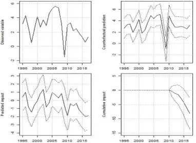
Figure 2 shows the plots of the shows the results of the posterior inference of the Causal Impact Analysis (CIA). The first graph shows the real GDP growth of South Africa and is the actual, or observed, variable. The real GDP growth of South Africa averaged about 4.1 percent between 2000 and 2008, it recorded a decline of about 1.5 percent in 2009 before rebounding to 3.3 percent where it subsequently sustained a persistent decrease recording 0.6 percent in 2016 and slight increase in 2017. The real GDP growth of South Africa never recovered to the levels recorded during the pre global financial crisis period. Although real GDP growth of South Africa underperformed its pre global financial crisis period levels, its trajectory was not vastly different from that of the other group of economies. In particular, the real GDP growth of Advanced economies is almost comparable to that of South Africa from 1995 to 2003 as well as towards the end of the sample period. Most economies experienced a significant decline in economic activity in 2009 where unprecedented economic stimulus packages were implemented to spur their economies out of recession, particularly in Advanced economies. Thus the economic policies in South Africa and most Emerging economies could have been deficient to advance real GDP growth and the economic activity to the levels of growth recorded during the pre global financial crisis period.

The second graph shows the plot of the unobserved synthetic baseline, or expected, data series. This is the counterfactual prediction which is the forecasted data series using the World real GDP growth as the surrogate, or control, variable. The unobserved synthetic baseline, or expected, data series is forecasted both in the training, or pre intervention, period and the period for computing a counterfactual prediction, or the post intervention period. The unobserved synthetic baseline, or expected, data series moves closely with the actual, or observed, real GDP growth of South Africa in the training, or pre intervention, period as expected. This close relationship is broken during the counterfactual prediction, or the post intervention period, which marks the post global financial crisis period. Thus the unobserved synthetic baseline, or expected, data series shows that the real GDP growth of South Africa could have been higher than the actual, or observed, real GDP growth. The lost output in the post intervention, or post global financial crisis, period confirms that perhaps the countercyclical macroeconomic policy intervention in South Africa did not achieve the desired results. Therefore, the economic stimulus to spur real GDP growth and economic activity to the pre global financial crisis levels could not be realised.

Notes: Own calculations using data from the International Monetary Fund (IMF) World Economic Outlook (WEO) database. The left hand scale measures the percentage causal impact. Observed variable is is the actual, or observed, real GDP growth. Counterfactual prediction is the unobserved synthetic baseline, or expected, data series. Predicted impact is the difference between the actual, or observed, variable and counterfactual prediction. Cumulative impact is the sum of the pointwise contributions from the Predicted impact that give a plot of the aggregate impact of the intervention.

The third graph shows the plot of the causal impact, which is the difference between the actual, or observed, variable and the synthetic baseline, or expected, data series. The predicted impact of real GDP growth fluctuated in the range of between positive 1.0 percent and negative 1.0 percent during the pre intervention period which coincides with the period before the onset of the global financial crisis. However, this changed during the period after the onset of the global financial crisis where the predicted impact fluctuated in the range of between -1.0 percent and -2.0 percent. The predicted affect shows that real GDP growth averaged about -0.5 percent between 2011 and 2013, real GDP growth deteriorated further between 2014 and 2017 almost recorded -2.0 percent in 2016 before it rebounded somewhat in 2017. The fourth graph is the plot of the cumulative impact, which is the sum of the Predicted impact data series since 2010. It shows that the cumulative real output loss was about -2.7 percent by 2014 while it increased to about -8.1 percent in 2017. This confirms that the trajectory of the the real output loss which accelerated significantly between 2014 and 2017 as shown by the predicted impact data series.

In summary, Descriptive Analysis (DA) and Bayesian Model Averaging (BMA) have shown that real GDP growth of South Africa largely moved in tandem with the World real GDP growth in the period pre global financial crisis. However, this close correlation in terms of size and temporal structure between the two variables changed post global financial crisis period in terms of size. In particular, the real GDP growth rate of South Africa was lower than World real GDP growth rate in this period. Causal Impact Analysis (CIA) revealed that real GDP growth of South Africa consistently recorded lower growth rates compared to the World real GDP growth during the post the global financial crisis period. The severity of the global financial crisis necessitated most economies, including South Africa, to implement unprecedented economic stimulus packages and other monetary and fiscal initiatives to recover economic performance from the widespread recessionary conditions. Thus the output loss in South Africa post the global financial crisis could be attributed to the deficiency of the countercyclical macroeconomic policies to restore the economic performance to levels recorded during the pre global financial crisis period.

Conclusion

This paper quantified economic recovery following the recent global financial crisis in South Africa. In particular, the paper measured the impact of the economic policy interventions that were implemented to spur the economy out of the recessionary conditions following the global financial crisis. The results show that real GDP growth recorded an average of 1.9 percent and a cumulative of 13.0 percent in the period post the global financial crisis. The counterfactual prediction shows that the economy could have potentially recorded the average real GDP growth of 3.0 percent and a cumulative of 21.0 percent in the period post the global financial crisis. Thus the causal impact of the economic policy interventions to spur the economy out of the recession since the global financial crisis is an average of -1.2 percent and a cumulative of -8.1 percent so that the relative impact of the post crisis policy intervention is -38.0 percent. The paper, therefore, concludes that perhaps the countercyclical macroeconomic policies in South Africa to advance output growth and the economy to the performance levels that were recorded during the pre global financial crisis period were deficient and hence such policies did not achieve the desired results.

References

Angrist, J. D. and Pischke, J.-S. (2008). Mostly Harmless Econometrics: An Empiricist’s Companion. Princeton university press.

Ashenfelter, O. and Card, D. (1985). Using the Longitudinal Structure of Earnings to Estimate the Effect of Training Programs. The Review of Economics and Statistics, 67(4):648–660.

Athey, S. and Imbens, G. W. (2006). Identification and Inference in Nonlinear Difference in Differences Models. Econometrica, 74(2):431–497.

Bartels, L. M. (1997). Specification Uncertainty and Model Averaging. American Journal of Political Science, 41(2):641–674.

Bordo, Michael and Eichengreen, Barry and Klingebiel, Daniela and Martinez-Peria, Maria Soledad (2001). Is the crisis problem growing more severe? Economic Policy, 16(32):52–82.

Chauvet, L. and Collier, P. (2008). What are the Preconditions for Turnarounds in Failing States?

Conflict Management and Peace Science, 25(4):332–348.

Dollar, D. and Svensson, J. (2000). What Explains the Success or Failure of Structural Adjustment Programmes? The Economic Journal, 110(466):894–917.

Feldkircher, M. and Zeugner, S. (2015). Bayesian Model Averaging Employing Fixed and Flexible Priors.

Journal of Statistical Software, 68(4):1–37.

Gambacorta, L., Hofmann, B., and Peersman, G. (2014). The Effectiveness of Unconventional Monetary Policy at the Zero Lower Bound: A Cross Country Analysis. Journal of Money, Credit and Banking, 46(4):615–642.

Gulde, A. M. and Schulze-Ghattas, M. (1993). Purchasing Power Parity Based Weights for the World Economic Outlook. International Monetary Fund Staff Studies, pages 106–120.

Harman, M., Martin, W., and Sarro, F. (2015). Causal Impact Analysis Applied to App Releases in Google Play and Windows Phone Store. Research Note, 15(07). UCL Department of Computer Science.

Harman, M., Martin, W., and Sarro, F. (2016). Causal Impact Analysis for App Releases in Google Play. In Zimmermann, T., Cleland-Huang, J., and Su, Z., editors, 24th ACM SIGSOFT Interna-tional Symposium on Foundations of Software Engineering, pages 435–446. Association for Computing Machinery.

Hoeting, J. A., Madigan, D., Raftery, A. E., and Volinsky, C. T. (1999). Bayesian Model Averaging: A Tutorial. Statistical Science, 44(4):382–401.

Imbens, G. and Wooldridge, J. (2007). Difference in Differences Estimation. Lecture Notes, 10. National Bureau of Economic Research Summer Institute.

IMF (2003). Unconventional Monetary Policies - Recent Experience and Prospects. International Mone-tary Fund (IMF).

Ishwaran, H. and Rao, J. S. (2005). Spike and Slab Variable Selection: Frequentist and Bayesian Strate-gies. The Annals of Statistics, 33(2):730–773.

Kapp, D. and Vega, M. (2014). Real Output Costs of Financial Crises: A Loss Distribution Approach.

Cuadernos de Economia, 37(103):13–28.

Leamer, E. E. (1978). Specification Searches: Ad Hoc Inference with Non Experimental Data. John Wiley and Sons Inc.

Mishkin, F. S. (2011). Over the cliff: From the Sub Prime to the Global Financial Crisis. Journal of Economic Perspectives, 25(1):49–70.

Mitchell, T. J. and Beauchamp, J. J. (1988). Bayesian Variable Selection in Linear Regression. Journal of the American Statistical Association, 83(404):1023–1032.

North, D. C. (1994). Economic Performance Through Time. The American Economic Review, 84(3):359– 368.

OECD (2010).Economic Surveys: South Africa, volume 2010/11. Organisation for Economic Cooperation and Development (OECD) Publishing.

Ruccio, D. (1993). The hidden successes of failed economic policies.Report on the Americas, 26(4):38–46.

Schularick, M. and Taylor, A. M. (2012). Credit Booms Gone Bust: Monetary Policy, Leverage Cycles and Financial Crises, 1870-2008. American Economic Review, 102(2):1029–61.

Taylor, J. B. (2013). Getting Off Track: How Government Actions and Interventions Caused, Prolonged and Worsened the Financial Crisis. Hoover Press.

Varian, H. R. (2014). Big Data: New Tricks for Econometrics. Journal of Economic Perspectives, 28(2):3–28.