User Modeling in Language Learning with Macaronic Texts
Adithya Renduchintala and Rebecca Knowles and Philipp Koehn and Jason Eisner Department of Computer Science
Johns Hopkins University
{adi.r,rknowles,phi,eisner}@jhu.edu
Abstract
Foreign language learners can acquire new vocabulary by using cognate and con-text clues when reading. To measure such incidental comprehension, we devise an experimental framework that involves reading mixed-language “macaronic” sen-tences. Using data collected via Ama-zon Mechanical Turk, we train a graphi-cal model to simulate a human subject’s comprehension of foreign words, based on cognate clues (edit distance to an English word), context clues (pointwise mutual in-formation), and prior exposure. Our model does a reasonable job at predicting which words a user will be able to understand, which should facilitate the automatic con-struction of comprehensible text for per-sonalized foreign language education.
1 Introduction
Second language (L2) learning requires the ac-quisition of vocabulary as well as knowledge of the language’s constructions. One of the ways in which learners become familiar with novel vocab-ulary and constructions is through reading. Ac-cording to Krashen’s Input Hypothesis (Krashen, 1989), learners acquire language through inciden-tal learning, which occurs when learners are ex-posed to comprehensible input. What constitutes “comprehensible input” for a learner varies as their knowledge of the L2 increases. For example, a student in their first month of German lessons would be hard-pressed to read German novels or even front-page news, but they might understand brief descriptions of daily routines. Comprehen-sible input need not be completely familiar to the learner; it could include novel vocabulary items or structures (whose meanings they can glean from context). Such input falls in the “zone of proxi-mal development” (Vygotski˘ı, 2012), just outside of the learner’s comfort zone. The related
con-cept of “scaffolding” (Wood et al., 1976) consists of providing assistance to the learner at a level that is just sufficient for them to complete their task, which in our case is understanding a sentence.
Automatic selection or construction of comprehensible input—perhaps online and personalized—would be a useful educational technology. However, this requires modeling the student: what can an L2 learner understand in a given context? In this paper, we develop a model and train its parameters on data that we collect.
For the remainder of the paper we focus on native English speakers learning German. Our methodology is a novel solution to the problem of controlling for the learner’s German skill level. We use subjects withzero previous knowledge of German, but we translate portions of the sentence into English. Thus, we can presume that theydo already know the English words and do not al-ready know the German words (except from see-ing them in earlier trials within our experiment). We are interested in whether they can jointly infer the meanings of the remaining German words in the sentence, so we ask them to guess.
The resulting stimuli are sentences like “Der Polizist arrested the Bankr¨auber.” Even a reader with no knowledge of German is likely to be able to understand this sentence reasonably well by us-ing cognate and context clues. We refer to this as amacaronicsentence; so-called macaronic lan-guage is a pastiche of two or more lanlan-guages (of-ten in(of-tended for humorous effect).
Our experimental subjects are required to guess what “Polizist” and “Bankr¨auber” mean in this sentence. We train a featurized model to pre-dict these guesses jointly within each sentence and thereby predict incidental comprehension on any macaronic sentence. Indeed, we hope our model design will generalize from predicting incidental comprehension on macaronic sentences (for our beginner subjects, who need some context words to be in English) to predicting incidental compre-hension on full German sentences (for more
vanced students, who understand some of the con-text wordsas ifthey were in English). In addition, we are developing a user interface that uses maca-ronic sentences directly as a medium of language instruction: our companion paper (Renduchintala et al., 2016) gives an overview of that project.
We briefly review previous work, then describe our data collection setup and the data obtained. Fi-nally, we discuss our model of learner comprehen-sion and validate our model’s predictions.
2 Previous Work
Natural language processing (NLP) has long been applied to education, but the majority of this work focuses on evaluation and assessment. Promi-nent recent examples include Heilman and Mad-nani (2012), Burstein et al. (2013) and MadMad-nani et al. (2012). Other works fall more along the lines of intelligent and adaptive tutoring systems designed to improve learning outcomes. Most of those are outside of the area of NLP (typically fo-cusing on math or science). An overview of NLP-based work in the education sphere can be found in Litman (2016). There has also been work spe-cific to second language acquisition, such as ¨Ozbal et al. (2014), where the focus has been to build a system to help learners retain new vocabulary. However, much of the existing work on incidental learning is found in the education and cognitive science literature rather than NLP.
Our work is related to Labutov and Lipson (2014), which also tries to leverage incidental learning using mixed L1 and L2 language. Where their work uses surprisal to choose contexts in which to insert L2 vocabulary, we consider both context features and other factors such as cognate features (described in detail in 4.1). We collect data that gives direct evidence of the user’s un-derstanding of words (by asking them to provide English guesses) rather than indirectly (via ques-tions about sentence validity, which runs the risk of overestimating their knowledge of a word, if, for instance, they’ve only learned whether it is an-imate or inanan-imate rather than the exact meaning). Furthermore, we are not only interested in whether a mixed L1 and L2 sentence is comprehensible; we are also interested in determining a distribution over the learner’s belief state for each word in the sentence. We do this in an engaging, game-like setting, which provides the user with hints when the task is too difficult for them to complete.
3 Data Collection Setup
Our method of scaffolding is to replace certain for-eign words and phrases with their English trans-lations, yielding a macaronic sentence.1 Simply presenting these to a learner would not give us feedback on the learner’s belief state for each for-eign word. Even assessing the learner’s reading comprehension would give only weak indirect in-formation about what was understood. Thus, we collect data where a learner explicitly guesses a foreign word’s translation when seen in the mac-aronic context. These guesses are then treated as supervised labels to train our user model.
We used Amazon Mechanical Turk (MTurk) to collect data. Users qualified for tasks by complet-ing a short quiz and survey about their language knowledge. Only users whose results indicated no knowledge of German and self-identified as native speakers of English were allowed to com-plete tasks. With German as the foreign language, we generated content by crawling a
simplified-German news website,nachrichtenleicht.
de. We chose simplified German in order to minimize translation errors and to make the task more suitable for novice learners. We translated each German sentence using the Moses Statis-tical Machine Translation (SMT) toolkit (Koehn et al., 2007). The SMT system was trained on the German-English Commoncrawl parallel text used in WMT 2015 (Bojar et al., 2015).
We used 200 German sentences, presenting each to 10 different users. In MTurk jargon, this yielded 2000 Human Intelligence Tasks (HITs). Each HIT required its user to participate in several rounds of guessing as the English translation was incrementally revealed. A user was paid US$0.12 per HIT, with a bonus of US$6 to any user who accumulated more than 2000 total points.
Our HIT user interface is shown in the video at
https://youtu.be/9PczEcnr4F8.
3.1 HITs and Submissions
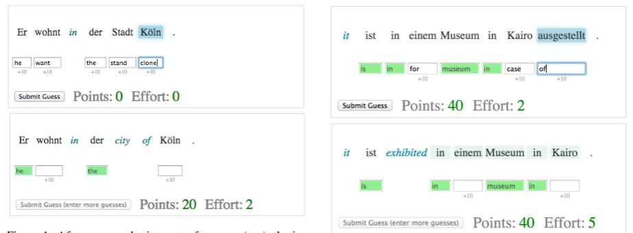
For each HIT, the user first sees a German sen-tence2 (Figure 1). A text box is presented below each German word in the sentence, for the user 1Although the language distinction is indicated by italics and color, users were left to figure this out on their own.
Figure 1: After a user submits a set of guesses (top), the in-terface marks the correct guesses in green and also reveals a set of translation clues (bottom). The user now has the oppor-tunity to guess again for the remaining German words.
to type in their “best guess” of what each Ger-man word means. The user must fill in at least half of the text boxes before submitting this set of guesses. The resultingsubmission—i.e., the maca-ronic sentence together with the set of guesses—is logged in a database as a single training example, and the system displays feedback to the user about which guesses were correct.
After each submission, new cluesare revealed (providing increased scaffolding) and the user is asked to guess again. The process continues, yielding multiple submissions, until all German words in the sentence have been translated. At this point, the entire HIT is considered completed and the user moves to a new HIT (i.e., a new sentence). From our 2000 HITs, we obtained 9392 submis-sions (4.7 per HIT) from 79 distinct MTurk users.
3.2 Clues
Each update provides new clues to help the user make further guesses. There are 2 kinds of clues:
Translation Clue(Figure 1): A set of words that were originally in German are replaced with their English translations. The text boxes below these words disappear, since it is no longer necessary to guess them.
Reordering Clue (Figure 2): A German sub-string is moved into a more English-like position. The reordering positions are calculated using the word and phrase alignments obtained from Moses. Each time the user submits a set of guesses, we reveal a sequence of n = max(1,round(N/3))
clues, whereN is the number of German words re-maining in the sentence. For each clue, we sample a token that is currently in German. If the token is
Figure 2: In this case, after the user submits a set of guesses (top), two clues are revealed (bottom): ausgestelltis moved into English order and then translated.
part of a movable phrase, we move that phrase; otherwise we translate the minimal phrase con-taining that token. These moves correspond ex-actly to clues that a user could request by clicking on the token in the macaronic reading interface of Renduchintala et al. (2016)—see that paper for de-tails of how moves are constructed and animated. In our present experiments, the system is in control instead, and grants clues by “randomly clicking” onntokens.
The system’s probability of sampling a given to-ken is proportional to its unigram type probability in the WMT corpus. Thus, rarer words tend to re-main in German for longer, allowing the Turker to attempt more guesses for these difficult words.
3.3 Feedback
When a user submits a set of guesses, the sys-tem responds with feedback. Each guess is vis-ibly “marked” in left-to-right order, momentarily shaded with green (for correct), yellow (for close) or red (for incorrect). Depending on whether a guess is correct, close, or wrong, users are awarded points as discussed below. Yellow and red shading then fades, to signal to the user that they may try entering a new guess. Correct guesses remain on the screen for the entire task.
3.4 Points
cor-rect translation, as measured by cosine similarity in vector space. (We used pre-trained GLoVe word vectors (Pennington et al., 2014); when the guess or correct translation has multiple words, we take the average of the word vectors.) We deduct effort points for guesses that are careless or very poor. Our rubric for effort points is as follows:
ep=
−1, ifˆeis repeated or nonsense (red)
−1, ifsim(ˆe, e∗)<0(red) 0, if0≤sim(ˆe, e∗)<0.4(red)
0, ifˆeis blank
10×sim(ˆe, e∗) otherwise (yellow)
Here sim(ˆe, e∗) is cosine similarity between the
vector embeddings of the user’s guess ˆeand our reference translatione∗. A “nonsense” guess
con-tains a word that does not appear in the sentence bitext nor in the 20,000 most frequent word types in the GLoVe training corpus. A “repeated” guess is an incorrect guess that appears more than once in the set of guesses being submitted.
In some cases,eˆore∗may itself consist of
mul-tiple words. In this case, our points and feedback are based on the best match between any word of
ˆ
eand any word ofe∗. In alignments where
mul-tiple German words translate as a single phrase,3 we take the phrasal translation to be the correct answere∗foreachof the German words.
3.5 Normalization
After collecting the data, we normalized the user guesses for further analysis. All guesses were lowercased. Multi-word guesses were crudely re-placed by the longest word in the guess (breaking ties in favor of the earliest word).
The guesses included many spelling errors as well as some nonsense strings and direct copies of the input. We defined thedictionary to be the 100,000 most frequent word types (lowercased) from the WMT English data. If a user’s guess ˆe does not matche∗ and is not in the dictionary, we
replace it with
• the special symbol <COPY>, if ˆe appears to be a copy of the German source word f (meaning that its Levenshtein distance from f is<0.2·max(|eˆ|,|f|));
• else, the closest word in the dictionary4 as measured by Levenshtein distance (breaking 3Our German-English alignments are constructed as in Renduchintala et al. (2016).
4Considering only words returned by the Pyenchant ‘sug-gest’ function (http://pythonhosted.org/pyenchant/).
ties alphabetically), provided the dictionary has a word at distance≤2;
• else<BLANK>, as if the user had not guessed.
4 User Model
In each submission, the user jointly guesses sev-eral English words, given spelling and context clues. One way that a machine could perform this task is via probabilistic inference in a factor graph—and we take this as our model of how the human usersolves the problem.
The user observes a German sentence f = [f1, f2, . . . , fi, . . . fn]. The translation of each word token fi is Ei, which is from the user’s point of view a random variable. Let Obs denote the set of indices i for which the user also ob-serves thatEi = e∗i, the aligned reference trans-lation, because e∗
i has already been guessed cor-rectly (green feedback) or shown as a clue. Thus, the user’s posterior distribution overEisPθ(E= e | EObs = e∗Obs,f,history), where “history” de-notes the user’s history of past interactions.
We assume that a user’s submissionˆeis derived from this posterior distribution simply as a ran-dom sample. We try to fit the parameter vector
θ to maximize the log-probability of the submis-sion. Note that our model is trained on the user guessesˆe, not the reference translationse∗. That is, we seek parametersθ that would explain why all users made their guesses.
Although we fit a single θ, this does not mean that we treat users as interchangeable (since θ
can include user-specific parameters) or unvary-ing (since our model conditions users’ behavior on their history, which can capture some learning).
4.1 Factor Graph
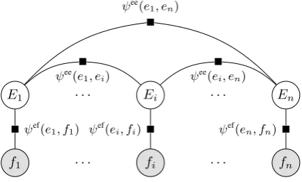
We model the posterior distribution as a condi-tional random field (Figure 3) in which the value of Ei depends on the form of fi as well as on the meaningsej (which may be either observed or jointly guessed) of the context words atj6=i:
Pθ(E=e|EObs=e∗Obs,f,history) (1)
∝ Y
i/∈Obs
(ψef(ei, fi)·Y
j6=i
ψee(ei, ej, i−j))
f1 . . . fi . . . fn
E1 . . . Ei . . . En
ψee(e
1, ei) ψee(ei, en)
ψee(e 1, en)
ψef(e
[image:5.595.73.290.66.197.2]1, f1) ψef(ei, fi) ψef(en, fn)
Figure 3: Model for user understanding of L2 words in sen-tential context. This figure shows an inference problem in which all the observed words in the sentence are in German (that is, Obs=∅). As the user observes translations via clues or correctly-marked guesses, some of theEibecome shaded.
factor ψef(ei, fi) considers whether the hypothe-sized English word ei “looks like” the observed German wordfi, and whether the user has previ-ously observed during data collection that ei is a correct or incorrect translation offi. Meanwhile, the factorψee(ei, ej)considers whethereiis com-monly seen in the context ofejin English text. For example, the user will elevate the probability that Ei = cakeif they are fairly certain thatEj is a related word likeeatorchocolate.
The potential functionsψare parameterized by
θ, a vector of feature weights. For convenience, we define the features in such a way that we ex-pect their weights to be positive. We rely on just 6 features at present (see section 6 for future work), although each is complex and real-valued. Thus, the weightsθ control the relative influence of these 6 different types of information on a user’s guess. Our features broadly fall under the follow-ing categories:Cognate,History, andContext. We precomputed cognate and context features, while history features are computed on-the-fly for each training instance. All features are case-insensitive. 4.1.1 Cognate and History Features
For each German tokenfi, theψeffactor can score each possible guesseiof its translation:
ψef(ei, fi) = exp(θef·φef(ei, fi)) (2)
The feature functionφefreturns a vector of 4 real numbers:
• Orthographic Similarity: The normalized Levenshtein distance between the 2 strings.
φeforth(ei, fi) = 1−max(lev(|ei, fiei|,|fi)|) (3)
The weight on this feature encodes how much users pay attention to spelling.
• Pronunciation Similarity: This feature is sim-ilar to the previous one, except that it cal-culates the normalized distance between the pronunciationsof the two words:
φefpron(ei, fi) =φorthef (prn(ei),prn(fi)) (4)
where the function prn(x) maps a string x to its pronunciation. We obtained pronuncia-tions for all words in the English and German vocabularies using the CMU pronunciation dictionary tool (Weide, 1998). Note that we use English pronunciation rules even for Ger-man words. This is because we are modeling a naive learner who may, in the absence of intuition about German pronunciation rules, apply English pronunciation rules to German.
• Positive History Feature: If a user has been rewarded in a previous HIT for guessing ei as a translation of fi, then they should be more likely to guess it again. We define
φef
hist+(ei, fi) to be 1 in this case and 0 oth-erwise. The weight on this feature encodes whether users learn from positive feedback.
• Negative History Feature: If a user has al-ready incorrectly guessedei as a translation of fi in a previous submission during this HIT, then they should be less likely to guess it again. We defineφefhist-(ei, fi)to be−1in this case and 0 otherwise. The weight on this fea-ture encodes whether users remember nega-tive feedback.5
4.1.2 Context Features
In the same way, theψef factor can score the com-patibility of a guess ei with a context word ej, which may itself be a guess, or may be observed:
ψeeij(ei, ej) = exp(θee·φee(ei, ej, i−j)) (5)
φeereturns a vector of 2 real numbers:
φee
pmi(ei, ej) =
(
PMI(ei, ej)if|i−j|>1
0otherwise (6)
φeepmi1(ei, ej) =
(
PMI1(ei, ej)if|i−j|= 1
0otherwise (7)
where the pointwise mutual information
PMI(x, y) measures the degree to which the English words x, y tend to occur in the same English sentence, and PMI1(x, y) measures how often they tend to occur in adjacent positions. These measurements are estimated from the English side of the WMT corpus, with smoothing performed as in Knowles et al. (2016).
For example, iffi =Suppe, the user’s guess of Eishould be influenced byfj =Brotappearing in the same sentence, if the user suspects or ob-serves that its translation is Ej = bread. The PMI feature knows that soup and bread tend to appear in the same English sentences, whereas PMI1knows that they tend not to appear in the
bi-gramsoup breadorbread soup.
4.1.3 User-Specific Features
Apart from the basic 6-feature model, we also trained a version that includes user-specific copies of each feature (similar to the domain adaptation technique of Daum´e III (2007)). For example, φef
orth,32(ei, fi) is defined to equal φeforth(ei, fi) for submissions by user 32, and defined to be 0 for submissions by other users.
Thus, with 79 users in our dataset, we learned
6 × 80 feature weights: a local weight vector for each user and a global vector of “backoff” weights. The global weightθef
orth is large if users in general reward orthographic similarity, while θef
orth,32 (which may be positive or negative) cap-tures the degree to which user 32 rewards it more or less than is typical. The user-specific features are intended to capture individual differences in incidental comprehension.
4.2 Inference
According to our model, the probability that the user guessesEi = ˆeiis given by a marginal prob-ability from the CRF. Computing these marginals is a combinatorial optimization problem that in-volves reasoning jointly about the possible values of each Ei (i /∈ Obs), which range over the En-glish vocabularyVe.
We employ loopy belief propagation (Murphy et al., 1999) to obtain approximate marginals over the variables E. Atree-based schedule for mes-sage passing was used (Dreyer and Eisner, 2009, footnote 22). We run 3 iterations with a new ran-dom root for each iteration.
We define the vocabulary Ve to consist of all reference translationse∗
i and normalized user
guesseseˆifrom our entire dataset (see section 3.5), about 5K types altogether including <BLANK> and<COPY>. We define the cognate features to treat <BLANK> as the empty string and to treat <COPY>asfi. We define the PMI of these spe-cial symbols with anyeto be the mean PMI withe of all dictionary words, so that they are essentially uninformative.
4.3 Parameter Estimation
We learn our parameter vectorθto approximately maximize the regularized log-likelihood of the users’ guesses:
X
logPθ(E= ˆe|EObs=e∗Obs,f,history)
−λ||θ||2 (8)
where the summation is over all submissions in our dataset. The gradient of each summand re-duces to a difference between observed and ex-pected values of the feature vectorφ= (φef,φee), summed over all factors in (1). The observed fea-tures are computed directly by settingE= ˆe. The expected features (which arise from the log of the normalization constant of (1)) are computed ap-proximately by loopy belief propagation.
We trained θ using stochastic gradient descent (SGD),6with a learning rate of0.1and regulariza-tion parameter of0.2. The regularization parame-ter was tuned on our development set.
5 Experimental Results
We divided our data randomly into 5550 training instances, 1903 development instances, and 1939 test instances. Each instance was a single submis-sion from one user, consisting of a batch of “si-multaneous” guesses on a macaronic sentence.
We noted qualitatively that when a large num-ber of English words have been revealed, particu-larly content words, the users tend to make better guesses. Conversely, when most context is Ger-man, we unsuprisingly see the user leave many guesses blank and make other guesses based on string similarity triggers. Such submissions are difficult to predict as different users will come up with a wide variety of guesses; our model there-fore resorts to predicting similar-sounding words. For detailed examples of this see Appendix A.
Model Recall at(dev) k Recall at(test) k
1 25 50 1 25 50
Basic 15.24 34.26 38.08 16.14 35.56 40.30
[image:7.595.306.528.61.246.2]User-Adapted 15.33 34.40 38.67 16.45 35.71 40.57
Table 1: Percentage of foreign words for which the user’s ac-tual guess appears in our top-klist of predictions, for models with and without user-specific features (k∈ {1,25,50}).
For each foreign word fi in a submission with i /∈ Obs, our inference method (section 4.2) pre-dicts a marginal probability distribution over a user’s guessesˆei. Table 1 shows our ability to pre-dict user guesses.7 Recall that this task is essen-tially a structured prediction task that does joint 4919-way classification of each German word. Roughly 1/3 of the time, our model’s top 25 words include the user’s exact guess.
However, the recall reported in Table 1 is too stringent for our educational application. We could give the model partial credit for predicting a synonym of the learner’s guesseˆ. More precisely, we would like to give the model partial credit for predicting when the learner will make a poor guess of the truthe∗—even if the model does not predict
the user’s specific incorrect guesseˆ.
To get at this question, we use English word em-beddings (as in section 3.4) as a proxy for the se-mantics and morphology of the words. We mea-sure the actual quality of the learner’s guess ˆe as its cosine similarity to the truth, sim(ˆe, e∗).
While quality of 1 is an exact match, and qual-ity scores> 0.75 are consistently good matches, we found quality of ≈ 0.6 also reasonable. Pairs such as (mosque, islamic) and (politics, government) are examples from the collected data with quality ≈ 0.6. As quality becomes <0.4, however, the relationship becomes tenuous, e.g., (refugee,soil).
Similarly, we measure the predicted quality as
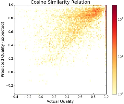
sim(e, e∗), where eis the model’s 1-best
predic-tion of the user’s guess. Figure 4 plots predicted vs. actual quality (each point represents one of the learner’s guesses on development data), ob-taining a correlation of 0.38, which we call the “quality correlation” or QC. A clear diagonal band can be seen, corresponding to the instances where 7Throughout this section, we ignore the 5.2% of tokens on which the user did not guess (i.e., the guess was<BLANK>
after the normalization of section 3.5). Our present model simply treats<BLANK>as an ordinary and very bland word (section 4.2), rather than truly attempting to predict when the user will not guess. Indeed, the model’s posterior probability of<BLANK>in these cases is a paltry 0.0000267 on average (versus 0.0000106 when the user does guess). See section 6.
Figure 4: Actual qualitysim(ˆe, e∗)of the learner’s guessˆeon development data, versus predicted qualitysim(e, e∗)where
[image:7.595.74.293.62.106.2]eis the basic model’s 1-best prediction.
Figure 5: Actual qualitysim(ˆe, e∗)of the learner’s guessˆe on development data, versus the expectation of the predicted qualitysim(e, e∗)whereeis distributed according to the ba-sic model’s posterior.
the model exactly predicts the user’s guess. The cloud around the diagonal is formed by instances where the model’s prediction was not identical to the user’s guess but had similar quality.
We also consider the expected predicted qual-ity, averaging over the model’s predictions e of
ˆ
e(for alle ∈ Ve) in proportion to the probabili-ties that it assigns them. This allows the model to more smoothly assess whether the learner is likely to make a high-quality guess. Figure 5 shows this version, where the points tend to shift upward and the quality correlation (QC) rises to 0.53.
[image:7.595.307.525.299.482.2]Model ExpDev1-Best ExpTest1-Best Basic 0.525 0.379 0.543 0.411
[image:8.595.79.286.62.106.2]User-Adapted 0.527 0.427 0.544 0.439 Table 2: Quality correlations: basic and user-adapted models.
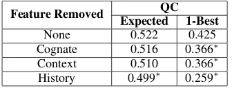
Feature Removed ExpectedQC 1-Best
None 0.522 0.425
Cognate 0.516 0.366∗
Context 0.510 0.366∗
[image:8.595.313.521.62.257.2]History 0.499∗ 0.259∗
Table 3: Impact on quality correlation (QC) of removing features from the model. Ablated QC values marked with asterisk∗differ significantly from the full-model QC values in the first row (p <0.05, using the test of Preacher (2002)).
5.1 Feature Ablation
To test the usefulness of different features, we trained our model with various feature categories disabled. To speed up experimentation, we sam-pled 1000 instances from the training set and trained our model on those. The resulting QC val-ues on dev data are shown in Table 3. We see that removing history-based features has the most sig-nificant impact on model performance: both QC measures drop relative to the full model. For cog-nate and context features, we see no significant im-pact on the expected QC, but a significant drop in the 1-best QC, especially for context features.
5.2 Analysis of User Adaptation
Table 2 shows that the user-specific features sig-nificantly improve the1-bestQC of our model, al-though the much smaller improvement inexpected QC is insignificant.
User adaptation allows us to discern differ-ent styles of inciddiffer-ental comprehension. A user-adapted model makes fine-grained predictions that could help to construct better macaronic sentences for a given user. Each user who completed at least 10 HITs has their user-specific weight vec-tor shown as a row in Figure 6. Recall that the user-specific weights are not used in isolation, but areaddedto backoff weights shared by all users.
These user-specific weight vectors cluster into four groups. Furthermore, the average points per HIT differ by cluster (significantly between each cluster pair), reflecting the success of different strategies.8Users in group (a) employ a generalist 8Recall that in our data collection process, we award points for each HIT (section 3.4). While the points were de-signed more as a reward than as an evaluation of learner suc-cess, a higher score does reflect more guesses that were
cor-Figure 6: The user-specific weight vectors, clustered into groups. Average points per HIT for the HITs completed by each group: (a) 45, (b) 48, (c) 50 and (d) 42.
strategy for incidental comprehension. They pay typical or greater-than-typical attention to all fea-tures of the current HIT, but many of them have diminished memory for vocabulary learned dur-ing past HITs (the hist+ feature). Users in group (b) seem to use the opposite strategy, deriving their success from retaining common vocabulary across HITs (hist+) and falling back on orthogra-phy for new words. Group (c) users, who earned the most points per HIT, appear to make heavy use of context and pronunciation featurestogether with hist+. We also see that pronunciation sim-ilarity seems to be a stronger feature for group (c) users, in contrast to the more superficial ortho-graphic similarity. Group (d), which earned the fewest points per HIT, appears to be an “extreme” version of group (b): these users pay unusually lit-tle attention to any model features other than or-thographic similarity and hist+. (More precisely, the model finds group (d)’s guesses harder to pre-dict on the basis of the available features, and so gives a more uniform distribution overVe.)
6 Future Improvements to the Model
[image:8.595.98.266.136.200.2]more plentiful and less noisy than the user guesses. For Cognate features, there exist many other good string similarity metrics (including trainable ones). We could also includeφeffeatures that con-sider whether ei’s part of speech, frequency, and length are plausible givenfi’s burstiness, observed frequency, and length. (E.g., only short common words are plausibly translated as determiners.)
For Contextfeatures, we could design versions that are more sensitive to the position and status of the context wordj. We speculate that the actual in-fluence ofej on a user’s guesseiis stronger when ej is observed rather than itself guessed; when there are fewer intervening tokens (and particu-larly fewer observed ones); and whenj < i. Or-thogonally, φef(ei, ej) could go beyond PMI and windowed PMI to also consider cosine similarity, as well as variants of these metrics that are thresh-olded or nonlinearly transformed. Finally, we do not have to treat the context positionsjas indepen-dent multiplicative influences as in equation (1) (cf. Naive Bayes): we could instead use a topic model or some form of language model to deter-mine a conditional probability distribution overEi given all other words in the context.
An obvious gap in our current feature set is that we have noφefeatures to capture that some words ei∈Veare more likely guessesa priori. By defin-ing several versions of this feature, based on fre-quencies in corpora of different reading levels, we could learn user-specific weights modeling which users are unlikely to think of an obscure word. We should also include features that fire specifi-cally on the reference translatione∗
i and the special symbols<BLANK>and<COPY>, as each is much more likely than the other features would suggest. For History features, we could consider nega-tivefeedback from other HITs (not just the current HIT), as well aspositiveinformation provided by revealed clues (not just confirmed guesses). We could also devise non-binary versions in which more recent or more frequent feedback on a word has a stronger effect. More ambitiously, we could model generalization: after being shown thatKindmeanschild, a learner might increase the probability that the similar word Kinder meanschildor something related (children, childish, . . . ), whether because of superficial orthographic similarity or a deeper understanding of the morphology. Similarly, a learner might gradually acquire a model of typical spelling
changes in English-German cognate pairs. A more significant extension would be to model a user’s learning process. Instead of represent-ing each user by a small vector of user-specific weights, we could recognize that the user’s guess-ing strategy and knowledge can change over time. A serious deficiency in our current model (not to mention our evaluation metrics!) is that we treat <BLANK>like any other word. A more at-tractive approach would be to learn a stochastic link from the posterior distribution to the user’s guess or non-guess, instead of assuming that the user simply samples the guess from the poste-rior. As a simple example, we might say the user guesses e ∈ Ve with probability p(e)β—where p(e) is the posterior probability andβ > 1 is a learned parameter—with the remaining probabil-ity assigned to<BLANK>. This says that the user tends to avoid guessing except when there are rel-atively high-probability words to guess.
7 Conclusion
We have presented a methodology for collecting data and training a model to estimate a foreign lan-guage learner’s understanding of L2 vocabulary in partially understood contexts. Both are novel con-tributions to the study of L2 acquisition.
Our current model is arguably crude, with only 6 features, yet it can already often do a reason-able job of predicting what a user might guess and whether the user’s guess will be roughly correct. This opens the door to a number of future direc-tions with applicadirec-tions to language acquisition us-ing personalized content and learners’ knowledge. We plan a deeper investigation into how learn-ers detect and combine cues for incidental com-prehension. We also leave as future work the in-tegration of this model into an adaptive system that tracks learner understanding and creates scaf-folded content that falls in their zone of prox-imal development, keeping them engaged while stretching their understanding.
Acknowledgments
References
Ondˇrej Bojar, Rajen Chatterjee, Christian Feder-mann, Barry Haddow, Matthias Huck, Chris Hokamp, Philipp Koehn, Varvara Logacheva, Christof Monz, Matteo Negri, Matt Post, Car-olina Scarton, Lucia Specia, and Marco Turchi. Findings of the 2015 Workshop on Statistical Machine Translation. In Proceedings of the Tenth Workshop on Statistical Machine Trans-lation, pages 1–46, 2015.
Jill Burstein, Joel Tetreault, and Nitin Madnani. The e-rater automated essay scoring system. In Mark D. Shermis, editor, Handbook of Auto-mated Essay Evaluation: Current Applications and New Directions, pages 55–67. Routledge, 2013.
Hal Daum´e III. Frustratingly easy domain adap-tation. InProceedings of ACL, pages 256–263, June 2007.
Markus Dreyer and Jason Eisner. Graphical mod-els over multiple strings. In Proceedings of EMNLP, pages 101–110, Singapore, August 2009.
Michael Heilman and Nitin Madnani. ETS: Dis-criminative edit models for paraphrase scoring. In Joint Proceedings of *SEM and SemEval, pages 529–535, June 2012.
Rebecca Knowles, Adithya Renduchintala,
Philipp Koehn, and Jason Eisner. Analyzing learner understanding of novel L2 vocabulary. 2016. To appear.
Philipp Koehn, Hieu Hoang, Alexandra Birch, Chris Callison-Burch, Marcello Federico, Nicola Bertoldi, Brooke Cowan, Wade Shen, Christine Moran, Richard Zens, Chris Dyer, Ondrej Bojar, Alexandra Constantin, and Evan Herbst. Moses: Open source toolkit for statistical machine translation. InProceedings of ACL: Short Papers, pages 177–180, 2007. Stephen Krashen. We acquire vocabulary and
spelling by reading: Additional evidence for the input hypothesis. The Modern Language Jour-nal, 73(4):440–464, 1989.
Igor Labutov and Hod Lipson. Generating code-switched text for lexical learning. In Proceed-ings of ACL, pages 562–571, 2014.
Diane Litman. Natural language processing for enhancing teaching and learning. In Proceed-ings of AAAI, 2016.
Nitin Madnani, Michael Heilman, Joel Tetreault, and Martin Chodorow. Identifying high-level organizational elements in argumentative dis-course. InProceedings of NAACL-HLT, pages 20–28, 2012.
Kevin P. Murphy, Yair Weiss, and Michael I. Jor-dan. Loopy belief propagation for approximate inference: An empirical study. InProceedings of UAI, pages 467–475, 1999.
G¨ozde ¨Ozbal, Daniele Pighin, and Carlo Strappa-rava. Automation and evaluation of the key-word method for second language learning. In Proceedings of ACL (Volume 2: Short Papers), pages 352–357, 2014.
Jeffrey Pennington, Richard Socher, and Christo-pher D. Manning. GLoVe: Global vectors for word representation. In Proceedings of EMNLP, volume 14, pages 1532–1543, 2014. K. J. Preacher. Calculation for the test of the
differ-ence between two independent correlation coef-ficients [computer software], May 2002. Benjamin Recht, Christopher Re, Stephen Wright,
and Feng Niu. Hogwild!: A lock-free ap-proach to parallelizing stochastic gradient de-scent. InAdvances in Neural Information Pro-cessing Systems, pages 693–701, 2011.
Adithya Renduchintala, Rebecca Knowles,
Philipp Koehn, and Jason Eisner. Creating interactive macaronic interfaces for language learning. In Proceedings of ACL (System Demonstrations), 2016.
Lev Vygotski˘ı. Thought and Language (Revised and Expanded Edition). MIT Press, 2012. R. Weide. The CMU pronunciation dictionary,
re-lease 0.6, 1998.
Appendices
A Example of Learner Guesses vs. Model Predictions
To give a sense of the problem difficulty, we have hand-picked and presented two training examples (submissions) along with the predictions of our basic model and their log-probabilities. In Figure 7a a large portion of the sentence has been revealed to the user in English (blue text) only 2 words are in German. The text in bold font is the user’s guess. Our model expected both words to be guessed; the predictions are listed below the German words VerschiedeneandRegierungen. The reference translation for the 2 words are Various and governments. In Figure 7b we see a much harder context where only one word is shown in English and this word is not particularly helpful as a contextual anchor.
(a)
(b)