Regional environmental efficiency in waste generation

(1)

Munich Personal RePEc Archive

Regional environmental efficiency in

waste generation

Halkos, George and Petrou, Kleoniki Natalia

Department of Economics, University of Thessaly

September 2017

Online at

https://mpra.ub.uni-muenchen.de/81237/

(2)

Regional environmental efficiency in waste generation

George Halkos and Kleoniki Natalia Petrou

_{Laboratory of Operations Research,}

Department of Economics, University of Thessaly

Abstract

This paper employs Data Envelopment Analysis (DEA) to consider waste generation at a regional level in the European Union (EU). By doing so both good and bad outputs are taken into account and different frameworks are designed. Five parameters (waste generation, employment rate, capital formation, GDP and population density) are used for 172 EU regions and for the years 2009, 2011 and 2013. In doing so four frameworks have been designed with different inputs and outputs each time. The results show the more efficient EU regions according to each framework, but it should be noted that results from different frameworks should not be compared to each other. Overall results suggest that the highest performers are regions in Belgium, Italy, Portugal and the UK. Finally the efficiency results from DEA were reviewed against the treatment options employed in the relevant regions. Our findings show that although a country might be efficient according to DEA and by taking many factors into consideration, it is not necessary that regions within a country use sustainable waste treatment options as it is essential to account for trade and shipment of waste between regions and countries as well.

Keywords: Environmental efficiency; waste generation; EU regions; DEA.

(3)

1. Introduction

Waste disposals have been increasing over the past few years, hence their management

has proved to be a rather challenging issue of the 21st_{century and a lot of research is being}

conducted in this field (Halkos and Petrou, 2016). Waste arisings and composition of waste

differs not only across countries, but also by region according but not limited to the following

factors (Eunomia, 2015): socioeconomic status, consumption habits, season, whether or not

households have gardens and presence (or not) of tourists. These factors have been analyzed

in various ways but most methods used in economic efficiency analysis are mainly

quantitative, although qualitative approaches (such as brainstorming, SWOT analysis, the

Delphi method) can be used too, usually to support quantitative findings attained through

(Soukopová, 2011):

a) Either single-criterion techniques: integrating several indicators into one (e.g. multiple

input-to-output ratios into a single efficiency score in the case of DEA)

b) Or multi-criteria analysis: keeping individual criteria separate to obtain a wider angle for

assessment, often including non-economic perspectives.

Our paper deals with waste generation at a regional level in the European Union and

employs Data Envelopment Analysis (DEA). By doing so both good and bad outputs are

taken into account and different frameworks are designed. Data Envelopment Analysis

(DEA) is a non-parametric approach that is used to measure the efficiency of certain Decision

Making Units (DMUs) by employing linear programming techniques (Boussofiane et al.,

1991). Then DEA assigns each DMU into an efficient frontier and produces an optimization

model which in turn produces lower values for the inputs and higher values for the outputs

(Lozano et al., 2009). DEA compares each DMU with all other and shows the ones that are

operating inefficiently compared to the others by identifying best practice scenarios (Sherman

(4)

above this one; therefore if there is a point where less input is consumed or more output is

produced then the DMU is considered inefficient (Lozano et al., 2009). The DEA frontier can

act as the production frontier, but it must be noted that DEA is a method for performance

evaluation and benchmarking against best-practice (Cook et al., 2014). DEA models treat bad

outputs in various ways. Specifically, undesirable outputs are treated as inputs for processing

(Berg et al., 1992; Hailu and Veeman, 2001), although this does not reflect the actual

production process (Seiford and Zhu, 2002); data for undesirable outputs are transformed and

those are used in evaluating environmental efficiency (Seiford and Zhu, 2002; Hua et al.,

2007); The disposability of the production technology is considered, which is suggested by

Fare et al. (1989; 1993; 2004; 2005) and further developed through other researchers too

(Tyteca, 1996; Zhou et al., 2008; Tone, 2001; Tone, 2004; Halkos and Tseremes, 2007).

In DEA the DMUs that are efficient are defined by a rating of 1 (or 100%) and these

ratings then form the efficiency frontier including the rest (not so efficient) DMUs; this rating

provides a realistic and practical value of what a certain DMU has achieved and what can be

further achieved by the other DMUs (Dostalova, 2014). Thus DEA disregards the ideal of

efficiency according to the economic theory and focuses mostly on real and so far-from-ideal

DMUs (Jablonský & Dlouhý, 2000). With time, extensions and additions have been done to

DEA modeling techniques. One of those that shows a good potential is Network DEA which

accounts for the relative efficiency of a system, by taking into account its whole structure

thus providing more informative and useful results (Kao, 2014).

2. Background

Some recent studies have employed DEA to evaluate the efficiency of waste management

(Bosch et al., 2000; Worthington and Dollery, 2001; Moore et al., 2005; Marques and Simões,

(5)

and Chen, 2012;). Further modifications are being made to DEA so that it can better capture

the full complexity of the process, for instance Rogge and De Jaeger (2012; 2013) suggested

a way to differentiate performance efficiency by the main municipal solid waste components.

Some regulating bodies and governments are using DEA also in their waste management

policies, such as Spain and Australia (Simões et al., 2010).

Most waste-related studies which employ DEA simply focus on waste or pollution as an

undesirable output within the standard DEA framework (Scheel, 2001; Seiford and Zhu,

2002). DEA has been also applied to measure the environmental performance at both micro

and macro levels (Kortelainen and Kuosmanen, 2005; frameworks by Sarkis, 1999; Zaim,

2004; chemical and pharmaceutical firms in Sueyoshi and Goto, 2014):

• investment into waste treatment technologies (Sarkis & Weinrach, 2001),

• waste prevention vs. ecological treatment and recycling (Sarkis & Cordeiro, 2001),

• carbon dioxide emissions on a national level (Ramanathan, 2002, 2005; Kumar,2006; Wang et al., 2012).

In this paper regional EU data (NUTS level 2) was used for 172 regions from 17 countries

and for the years 2009, 2011 and 2013.1_{According to the 1961 Brussels Conference on}

Regional Economies, NUTS 2 regional classification2_{is the most common framework used}

by Member States to apply their regional policies and therefore is the most appropriate level

for analysing regional environmental problems (Eurostat, 2007). The parameters used, are

counted as presented below:

 Regional waste arisings: waste generated (thousand tonnes)

 Regional employment rate: thousand number of people

 Regional gross fixed capital formation: current prices (million €)

1_{Regions (in parentheses) examined by country are Austria (7), Belgium (11), Bulgaria (6), Czech Republic (9),}

Estonia (1), Germany (36), Hungary (6), Italy (21), Latvia (1), Lithuania (1), Luxembourg (1), Malta (1), Netherlands (12), Poland (16), Portugal (7), Slovakia (4), UK (33).

(6)

 Regional GDP (as proxy of economic development) 3_{: current prices (million €)}

 Regional population density: persons per km2

2.1 Overall issues regarding missing variables in the current analysis

An issue that arose in the current analysis was that some data were missing in the

regional statistics for DEA. This created some problems in analysing and contrasting data

among different countries/regions.

In order to be able to handle missing data, it is vital to know why they are missing; there

are three general ‘missingness mechanisms’ (Gelman and Hill, 2007; IDRE, 2016):

 Missing completely at random (MCAR): neither the unobserved values of the variable

with missing nor the other variables in the dataset predict whether a value will be missing.

 Missing at random (MAR): other variables (but not the variable with missing itself) in the

dataset can be used to predict missingness.

 Missing not at random (MNAR): the unobserved value of the variable with missing

predicts missingness.

As far as this DEA analysis is concerned, the following assumptions had to be made to

replace some missing values in the regional data:

1. Data on waste arising for the UK were missing for 2013 and as waste is the most

important parameter in question for this project, it was assumed that waste arisings

remained the same between 2011 and 2013.

2. Data on population density were missing for Leipzig and Thüringen for 2009, so 2011

data were used.

3. Also data for population density were missing for Nord-Est and Zuid-Nederland for all

the examined years. To resolve this for Nord-Est the sum of Emilia-Romagna,

3_{For the determinants of the environment and development relationship see among others Halkos (1992, 2003,}

(7)

Venezia Giulia and Trentino-Alto Adige e Veneto was used as Nord-Est consists of these

regions. For Zuid-Nederland the relevant country’s average was used.

3. DEA modeling results – Regional level (17 EU countries, 172 regions)

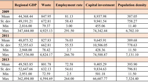
Table 1 presents the descriptive statistics of the inputs and outputs used in the different

[image:7.595.73.568.259.533.2]

DEA model formulations and for all the years in question for the 172 regions.

Table 1: Descriptive statistics for all years and regions

_{Regional GDP Waste Employment rate Capital investment Population density}

2009

Mean 44,368.44 847.95 81.13 8,937.98 387.05

St. dev 49,191.21 672.81 58.43 9,941.54 758.27

Min 2,816.00 79.37 3.00 455.06 11.40

Max 347,444.00 4,925.13 291.50 74,342.44 6,702.10

2011

Mean 48,075.32 827.83 76.03 9,645.91 389.68

St. dev 52,355.63 662.81 55.53 10,506.05 778.63

Min 2,948.00 78.42 2.7 428.36 11.50

Max 367,536.00 4,824.17 266.70 74,588.87 7,131.10

2013

Mean 49,583.85 801.78 72.58 9,405.29 393.90

St. dev 52,647.66 632.13 54.61 9,834.63 796.81

Min 2,951.00 72.59 2.5 501.18 11.50

Max 362,494.00 4,594.69 264.00 66,607.77 7,324.40

3.1 Presentation of four environmental production frameworks on regional analysis

The present analysis builds on the work by Halkos and Papageorgiou (2014, 2015)

and furthers it by using more inputs and outputs and more recent EU data. The frameworks

that have been designed are also based on their analysis with new additions in the inputs

taken into account. More specifically in terms of methodology, first one of the pollutants in

question, MSW generation is modelled as a regular output by applying the transformation

introduced by Seiford and Zhu (2002, 2005). This is done in the first framework (M1). Then

(8)

the main goal is its minimisation, which is performed in M2 and M3 each time with slightly

different inputs. In Framework M4 the idea of eco-efficiency is used as introduced by

Kuosmanen and Kortelainen (2005) and Kortelainen (2008). For all the regions in the DEA

analysis a radial model was used, which is output oriented and with variable returns to scale.

3.2 Results of the DEA regional level study

Under the M1 framework the highest performers over the years 2009-2013 are: Région de

Bruxelles-Capitale (Belgium), Yuzhen tsentralen (Bulgaria), Düsseldorf (Germany), Valle

d'Aosta (Italy), Liguria (Italy), Lombardia (Italy), Nord-Est (Italy), Lazio (Italy), Sicilia (Italy),

Luxembourg (Luxembourg), Algarve (Portugal), Greater Manchester (UK), Surrey, East and

West Sussex (UK); whereas the areas with the lowest performers are: Flevoland (Netherlands),

North Eastern Scotland (UK), Severozápad (Bulgaria), Zeeland (Netherlands), Trier (Germany),

Jihozápad (Czech Republic), Strední Cechy (Czech Republic), Eesti (Estonia), Highlands and

Islands (UK), Moravskoslezsko (Czech Republic), Prague (Czech Republic).

When using framework M2 and by treating the bad output as input, the highest

performers are: Bremen (Germany), Greater Manchester (UK), Luxembourg (Luxembourg),

Région de Bruxelles-Capitale (Belgium), Düsseldorf (Germany), Valle d'Aosta (Italy),

Lombardia (Italy), Nord-Est (Italy), Lazio (Italy), Surrey, East and West Sussex (UK). The

lowest performers are: Yugoiztochen (Bulgaria), Strední Cechy (Czech Republic), Severozápad

(Czech Republic), Highlands and Islands (UK), Dél-Dunántúl (Hungary), Zeeland (Netherlands),

North Eastern Scotland (UK), Észak-Alföld (Hungary), Yugozapadna i yuzhna tsentralna

(Bulgaria) and Flevoland (Netherlands).

Framework M3 is similar to M2 but with the addition of an extra parameter, population

density. In this one the highest performers are: Region de Bruxelles-Capitale (Belgium),

Severozapaden (Bulgaria), Düsseldorf (Germany), Valle d'Aosta/Vallée d'Aoste (Italy),

(9)

Luxembourg (Luxembourg), Zuid-Nederland (Nerherlands), Região Autónoma dos Açores

(Portugal), Surrey, East and West Sussex and Highlands and Islands (both UK). Under this

framework the worse performers are: Flevoland (Netherlands), Severozápad (Czech Republic),

Strední Cechy (Czech Republic), Zeeland (Netherlands), Moravskoslezsko (Czech Republic),

Yugoiztochen (Bulgaria), Dél-Dunántúl (Hungary), Észak-Alföld (Hungary), Podkarpackie

(Poland), Nyugat-Dunántúl (Hungary) and Praha (Czech Republic).

From framework M4, the highest performers are: Lombardia (Italy), Valle d'Aosta (Italy),

Nord-Est (Italy), whereas the lowest ones are: Severozapaden (Bulgaria), Severen tsentralen

(Bulgaria), Severoiztochen (Bulgaria), Yugoiztochen (Bulgaria), Yuzhen tsentralen (Bulgaria),

Dél-Dunántúl (Hungary), Malta (Malta), Észak-Magyarország (Hungary), Algarve (Portugal),

Opolskie (Poland).

As it is evident from this analysis, different frameworks return different results, namely

the results from M1 are much different to M2, M3 and M4 which show a kind of similar picture

overall. This difference can be explained by the fact that in M1 the bad output (waste generation)

is actually considered as output, whereas in the other three frameworks it is considered as a

normal input. Table 2 shows the average scores of each region for all the years divided by the

framework option.4

The results of each framework cannot be compared to each other though as different

assumptions are taken into account under each modelling framework. According to EEA (European

Environment Agency, 2015) and other researchers, there are fluctuations in waste generation not only

among the countries but also among regions within a country, which is due to the fact that there are

separate waste management strategies among the regions themselves as well. This study’s results are

in agreement with this idea, as it was shown that certain regions from one country can be at the top

environmental performers whereas other regions from the same one can be among the lowest ones.

4_{The Table presenting in detail the results of M1, M2, M3 and M4 frameworks for all regions for years 2009,}

(10)

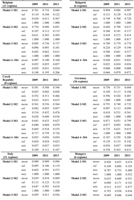
Furthermore table 3 presents the descriptive statistics per country of the different

environmental frameworks over the examined period. The results show that on average terms

the environmental efficiency scores regarding waste arising on a regional level are higher in

framework M1 compared to the environmental efficiency scores from M2, M3 and M4.

Overall the results obtained (on average terms) from M1 suggest that Belgium has higher

[image:10.595.72.531.256.758.2]

environmental efficient regions followed by the regions in Italy, Portugal and the UK.

Table 2: Average scores of each region for all the years divided by framework

M1 M2 M3 M4

Region Average Average Average Average

Région de Bruxelles-Capitale / Brussels Hoofdstedelijk Gewest 1.000 1.000 1.000 0.193

Prov. Antwerpen 0.694 0.723 0.775 0.196

Prov. Limburg (BE) 0.636 0.622 0.672 0.065

Prov. Oost-Vlaanderen 0.620 0.627 0.679 0.125

Prov. Vlaams-Brabant 0.729 0.729 0.806 0.110

Prov. West-Vlaanderen 0.602 0.604 0.658 0.105

Prov. Brabant Wallon 0.709 0.715 0.769 0.078

Prov. Hainaut 0.749 0.721 0.772 0.081

Prov. Liège 0.712 0.703 0.763 0.075

Prov. Luxembourg (BE) 0.722 0.687 0.779 0.032

Prov. Namur 0.682 0.682 0.754 0.044

Severozapaden 0.935 0.887 1.000 0.008

Severen tsentralen 0.991 0.887 0.948 0.009

Severoiztochen 0.872 0.587 0.656 0.012

Yugoiztochen 0.848 0.479 0.577 0.014

Yugozapadna i yuzhna tsentralna Bulgaria 0.729 0.533 0.658 0.069

Yuzhen tsentralen 1.000 0.606 0.687 0.016

Praha 0.570 0.605 0.634 0.109

Strední Cechy 0.550 0.488 0.563 0.047

Jihozápad 0.547 0.545 0.711 0.044

Severozápad 0.528 0.503 0.563 0.036

Severovýchod 0.638 0.620 0.722 0.051

Jihovýchod 0.576 0.562 0.666 0.064

Strední Morava 0.600 0.569 0.636 0.041

Moravskoslezsko 0.564 0.540 0.576 0.043

Stuttgart 0.740 0.771 0.822 0.454

Karlsruhe 0.752 0.794 0.833 0.279

Freiburg 0.676 0.727 0.810 0.191

Tübingen 0.630 0.698 0.772 0.173

Oberbayern 0.687 0.705 0.926 0.569

Niederbayern 0.694 0.748 0.896 0.104

Oberpfalz 0.637 0.701 0.829 0.099

Oberfranken 0.744 0.747 0.871 0.088

(11)

Unterfranken 0.752 0.787 0.916 0.119

Schwaben 0.643 0.688 0.782 0.162

Berlin 0.832 0.857 0.857 0.297

Brandenburg 0.664 0.689 0.862 0.160

Bremen 0.927 0.965 0.965 0.077

Hamburg 0.734 0.792 0.812 0.267

Darmstadt 0.864 0.902 0.925 0.462

Gießen 0.703 0.719 0.789 0.083

Kassel 0.720 0.744 0.862 0.103

Mecklenburg-Vorpommern 0.617 0.641 0.827 0.101

Braunschweig 0.661 0.686 0.767 0.149

Hannover 0.808 0.810 0.887 0.188

Lüneburg 0.633 0.627 0.767 0.108

Weser-Ems 0.629 0.649 0.753 0.199

Düsseldorf 1.000 1.000 1.000 0.510

Köln 0.889 0.900 0.932 0.426

Münster 0.788 0.795 0.839 0.207

Detmold 0.801 0.849 0.892 0.181

Arnsberg 0.895 0.905 0.944 0.297

Koblenz 0.706 0.716 0.815 0.116

Trier 0.538 0.570 0.662 0.037

Rheinhessen-Pfalz 0.697 0.705 0.758 0.175

Saarland 0.836 0.839 0.882 0.087

Dresden 0.579 0.640 0.695 0.109

Chemnitz 0.668 0.725 0.775 0.094

Leipzig 0.642 0.715 0.753 0.072

Thüringen 0.649 0.676 0.801 0.138

Eesti 0.553 0.547 0.873 0.046

Piemonte 0.778 0.795 0.936 0.345

Valle d'Aosta/Vallée d'Aoste 1.000 1.000 1.000 1.000

Liguria 1.000 0.884 0.933 0.130

Lombardia 1.000 1.000 1.000 0.958

Nord-Est 1.000 1.000 1.000 1.000

Provincia Autonoma di Bolzano/Bozen 0.616 0.629 0.763 0.055

Veneto 0.844 0.867 0.904 0.406

Friuli-Venezia Giulia 0.803 0.772 0.851 0.097

Emilia-Romagna 0.953 0.887 1.000 0.393

Toscana 0.988 0.941 1.000 0.297

Umbria 0.875 0.811 0.883 0.061

Marche 0.897 0.849 0.917 0.111

Lazio 1.000 1.000 1.000 0.513

Abruzzo 0.744 0.653 0.720 0.087

Molise 0.932 0.894 0.943 0.054

Campania 0.995 0.923 0.931 0.282

Puglia 0.922 0.828 0.869 0.196

(12)

Calabria 0.889 0.696 0.750 0.091

Sicilia 1.000 0.919 0.955 0.246

Sardegna 0.892 0.767 0.954 0.093

Latvija 0.674 0.562 0.889 0.057

Lietuva 0.962 0.702 0.979 0.086

Luxembourg 1.000 0.989 1.000 0.116

Közép-Magyarország 0.887 0.863 0.892 0.133

Nyugat-Dunántúl 0.784 0.551 0.626 0.027

Dél-Dunántúl 0.800 0.515 0.606 0.018

Észak-Magyarország 0.824 0.585 0.650 0.020

Észak-Alföld 0.845 0.528 0.610 0.026

Dél-Alföld 0.771 0.549 0.654 0.024

Malta 0.767 0.824 0.824 0.020

Groningen 0.868 0.922 0.961 0.082

Friesland (NL) 0.679 0.647 0.687 0.049

Drenthe 0.732 0.702 0.735 0.037

Overijssel 0.658 0.702 0.718 0.099

Gelderland 0.691 0.640 0.675 0.180

Flevoland 0.466 0.539 0.555 0.042

Utrecht 0.694 0.766 0.777 0.157

Noord-Holland 0.850 0.906 0.907 0.350

Zuid-Holland 0.741 0.766 0.767 0.380

Zeeland 0.532 0.525 0.569 0.031

Zuid-Nederland 0.745 0.808 1.000 0.360

Limburg (NL) 0.682 0.713 0.726 0.097

Wien 0.713 0.734 0.739 0.221

Kärnten 0.657 0.686 0.900 0.047

Steiermark 0.626 0.663 0.844 0.108

Oberösterreich 0.665 0.701 0.845 0.144

Salzburg 0.625 0.669 0.832 0.062

Tirol 0.583 0.615 0.819 0.075

Vorarlberg 0.693 0.894 0.909 0.087

Lódzkie 0.739 0.589 0.688 0.062

Mazowieckie 0.831 0.740 0.890 0.219

Malopolskie 0.800 0.663 0.713 0.078

Slaskie 0.932 0.688 0.713 0.129

Lubelskie 0.665 0.600 0.740 0.040

Podkarpackie 0.581 0.546 0.623 0.039

Swietokrzyskie 0.636 0.700 0.781 0.028

Podlaskie 0.634 +0.592 0.770 0.023

Wielkopolskie 0.838 0.694 0.851 0.096

Zachodniopomorskie 0.758 0.612 0.741 0.038

Lubuskie 0.673 0.624 0.724 0.022

Dolnoslaskie 0.791 0.649 0.761 0.085

Opolskie 0.687 0.687 0.753 0.022

Kujawsko-Pomorskie 0.736 0.601 0.706 0.045

(13)

Norte 0.888 0.706 0.818 0.138

Algarve 1.000 0.761 0.843 0.020

Centro (PT) 0.863 0.761 0.932 0.091

Área Metropolitana de Lisboa 0.969 0.926 0.932 0.181

Alentejo 0.729 0.623 0.976 0.031

Região Autónoma dos Açores (PT) 0.932 0.946 1.000 0.026

Região Autónoma da Madeira (PT) 0.927 0.9F08 0.908 0.038

Bratislavský kraj 0.603 0.599 0.670 0.054

Západné Slovensko 0.765 0.693 0.798 0.062

Stredné Slovensko 0.686 0.647 0.801 0.038

Východné Slovensko 0.705 0.676 0.796 0.039

Tees Valley and Durham 0.765 0.712 0.714 0.067

Northumberland and Tyne and Wear 0.798 0.772 0.798 0.090

Cumbria 0.803 0.828 0.983 0.034

Greater Manchester 1.000 0.986 0.986 0.186

Lancashire 0.937 0.910 0.917 0.091

East Yorkshire and Northern Lincolnshire 0.872 0.855 0.864 0.060

North Yorkshire 0.844 0.832 0.981 0.059

South Yorkshire 0.797 0.797 0.797 0.078

West Yorkshire 0.947 0.943 0.943 0.156

Derbyshire and Nottinghamshire 0.848 0.812 0.813 0.138

Leicestershire, Rutland and Northamptonshire 0.819 0.816 0.827 0.123

Lincolnshire 0.650 0.642 0.746 0.043

Herefordshire, Worcestershire and Warwickshire 0.790 0.786 0.826 0.092

Shropshire and Staffordshire 0.877 0.850 0.881 0.097

West Midlands 0.960 0.922 0.922 0.180

East Anglia 0.678 0.694 0.807 0.181

Bedfordshire and Hertfordshire 0.886 0.902 0.916 0.147

Essex 0.897 0.890 0.893 0.116

Berkshire, Buckinghamshire and Oxfordshire 0.839 0.885 0.915 0.253

Surrey, East and West Sussex 1.000 1.000 1.000 0.234

Hampshire and Isle of Wight 0.716 0.762 0.771 0.159

Kent 0.874 0.856 0.865 0.115

Gloucestershire, Wiltshire and Bristol/Bath area 0.817 0.840 0.910 0.200

Dorset and Somerset 0.837 0.835 0.885 0.086

Cornwall and Isles of Scilly 0.706 0.705 0.735 0.031

Devon 0.787 0.778 0.851 0.073

West Wales and The Valleys 0.853 0.752 0.893 0.100

East Wales 0.791 0.779 0.891 0.078

Eastern Scotland 0.778 0.732 0.917 0.153

South Western Scotland 0.757 0.687 0.822 0.159

North Eastern Scotland 0.479 0.526 0.691 0.057

Highlands and Islands 0.555 0.512 1.000 0.032

(14)

[image:14.595.63.530.83.778.2]

Table 3: Descriptive statistics of regions’ environmental efficiency estimates grouped by country Belgium

(11 regions) 2009 2011 2013 (6 regions) Bulgaria 2009 2011 2013

Model 1-M1 mean _{0.761 0.716 0.666} Model 1-M1 mean 0.894 0.886 0.907

std 0.110 0.104 0.122 std 0.121 0.128 0.120

min 0.628 0.611 0.567 min 0.749 0.700 0.720

max _{1.000 1.000 1.000} max 1.000 1.000 1.000

Model 2-M2 mean 0.754 0.686 0.691 Model 2-M2 mean 0.668 0.708 0.613

std 0.107 0.112 0.115 std 0.260 0.181 0.137

min 0.631 0.583 0.585 min 0.439 0.572 0.414

max 1.000 1.000 1.000 max 1.000 1.000 0.817

std 0.096 0.093 0.101 std 0.226 0.129 0.196

min 0.682 0.662 0.631 min 0.508 0.661 0.517

max 1.000 1.000 1.000 max 1.000 1.000 1.000

Model 4 -M4 mean 0.097 0.100 0.104 Model 4 -M4 mean 0.020 0.021 0.022

std _{0.052 0.053 0.057} std 0.022 0.024 0.024

min 0.029 0.031 0.034 min 0.008 0.008 0.008

max 0.188 0.195 0.206 max 0.066 0.070 0.071 Czech

Republic

(8 regions) 2009 2011 2013

Germany

(36 regions) 2009 2011 2013

std 0.025 0.042 0.056 std 0.109 0.113 0.104

min 0.552 0.511 0.466 min 0.596 0.526 0.487

max 0.632 0.651 0.633 max 1.000 1.000 1.000

std _{0.042 0.055 0.057} std 0.097 0.113 0.096

min 0.514 0.452 0.476 min 0.618 0.531 0.561

max 0.628 0.609 0.636 max 1.000 1.000 1.000

std 0.040 0.084 0.078 std 0.077 0.092 0.081

min _{0.605 0.524 0.535} min 0.735 0.621 0.615

max 0.717 0.759 0.726 max 1.000 1.000 1.000

std 0.024 0.024 0.023 std 0.129 0.133 0.142

min 0.037 0.037 0.035 min 0.036 0.037 0.040

max _{0.109 0.111 0.107} max 0.530 0.563 0.613 Italy

(21 regions) 2009 2011 2013 (6 regions) Hungary 2009 2011 2013

Model 1-M1 mean _{0.909 0.909 0.896} Model 1-M1 mean _{0.928 0.853 0.674}

std 0.095 0.106 0.119 std 0.104 0.086 0.183

min _{0.682 0.591 0.573} min _{0.787 0.753 0.480} max 1.000 1.000 1.000 max _{1.000 1.000 0.932}

std _{0.113 0.123 0.116} std _{0.098 0.171 0.141} min 0.647 0.593 0.618 min 0.512 0.527 0.477

(15)

std 0.094 0.082 0.092 std _{0.094 0.146 0.116} min 0.692 0.732 0.696 min 0.562 0.596 0.548

max _{1.000 1.000 1.000} max _{0.828 0.980 0.868}

std 0.314 0.315 0.315 std 0.045 0.045 0.045

min 0.034 0.038 0.038 min _{0.018 0.017 0.018} max 1.000 1.000 1.000 max 0.133 0.132 0.135 Netherlands

(12 regions) 2009 2011 2013 (7 regions) Austria 2009 2011 2013

std _{0.095 0.145 0.110} std 0.048 0.055 0.050

min 0.478 0.437 0.484 min 0.630 0.583 0.535

max _{0.827 1.000 0.896} max 0.755 0.727 0.695

std 0.116 0.154 0.110 std 0.116 0.115 0.048

min _{0.504 0.490 0.575} min 0.641 0.592 0.614

max 0.865 1.000 0.933 max 0.994 0.938 0.751

std 0.134 0.165 0.125 std 0.090 0.062 0.029

min 0.585 0.490 0.590 min 0.749 0.738 0.732

max _{1.000 1.000 1.000} max 1.000 0.938 0.820

std _{0.135 0.131 0.135} std 0.059 0.059 0.062

min 0.030 0.031 0.031 min 0.046 0.047 0.049

max 0.389 0.371 0.380 max 0.218 0.218 0.229 Poland

(16 regions) 2009 2011 2013 (7 regions) Portugal 2009 2011 2013

std 0.105 0.122 0.082 std 0.094 0.110 0.092

min 0.619 0.532 0.560 min 0.739 0.690 0.760

max _{1.000 0.908 0.890} max 1.000 1.000 1.000

std 0.077 0.098 0.071 std 0.145 0.156 0.109

min 0.468 0.435 0.525 min 0.612 0.544 0.714

max 0.788 0.785 0.768 max 1.000 1.000 1.000

std 0.080 0.096 0.084 std 0.098 0.075 0.059

min 0.544 0.560 0.606 min 0.717 0.810 0.844

max 0.840 0.949 0.909 max 1.000 1.000 1.000

std _{0.046 0.053 0.056} std 0.068 0.063 0.060

min 0.020 0.022 0.023 min 0.021 0.020 0.020

max 0.192 0.225 0.241 max 0.191 0.180 0.173 Slovakia

(4 regions) 2009 2011 2013 (33 regions) UK 2009 2011 2013

std 0.075 0.086 0.166 std 0.109 0.136 0.138

(16)

max 0.764 0.762 0.843 max 1.000 1.000 1.000

std _{0.061 0.048 0.144} std 0.116 0.136 0.133

min 0.614 0.535 0.502 min 0.537 0.403 0.361

max 0.759 0.634 0.820 max 1.000 1.000 1.000

std 0.073 0.067 0.196 std 0.096 0.110 0.101

min _{0.685 0.618 0.530} min 0.628 0.510 0.565

max 0.862 0.769 0.953 max 1.000 1.000 1.000

std 0.011 0.012 0.012 std 0.054 0.057 0.064

min 0.036 0.038 0.040 min 0.029 0.030 0.034

max _{0.059 0.062 0.065} max 0.229 0.249 0.280 4. Discussion

The efficiency scores obtained through DEA have been reviewed against the

treatment options that have been employed in each region and which for this analysis are

divided in landfill, incineration, material recycling and composting. Data for the treatment

options have been obtained from Eurostat as well. First of all it is worth mentioning that

overall in the EU a decrease in the use of landfill and an increase in the use of more

[image:16.595.99.499.504.715.2]

sustainable treatment options has been noticed over the period 1995-2015.

(17)

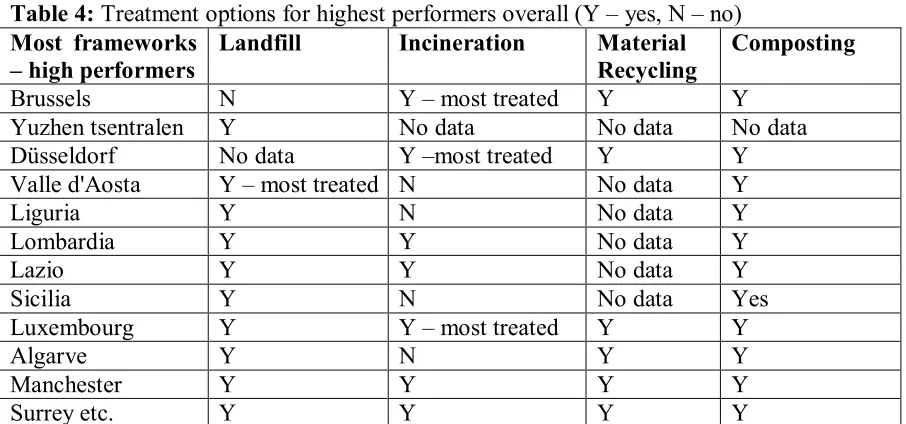
The aim of the comparison in this analysis was to investigate whether regions with the

use of more sustainable treatment options are the ones that are the highest performers

regarding efficiency based on the DEA analysis. Table 4 presents the treatment options that

have been used for the highest performing regions, whereas table 5 presents those options for

[image:17.595.67.520.224.436.2]

the lowest performers.5

Table 4: Treatment options for highest performers overall (Y – yes, N – no) Most frameworks

– high performers Landfill Incineration Material Recycling Composting

Brussels N Y – most treated Y Y

Yuzhen tsentralen Y No data No data No data

Düsseldorf No data Y –most treated Y Y

Valle d'Aosta Y – most treated N No data Y

Liguria Y N No data Y

Lombardia Y Y No data Y

Lazio Y Y No data Y

Sicilia Y N No data Yes

Luxembourg Y Y – most treated Y Y

Algarve Y N Y Y

Manchester Y Y Y Y

Surrey etc. Y Y Y Y

Table 5: Treatment options for lowest performers overall (Y – yes, N – no) Most frameworks –

lowest performers Landfill Incineration Material Recycling Composting

Severozápaden Y No data No data No data

Zeeland Y Y – most treated Y Y

Flevoland Y Y – most treated Y y

Strední Cechy No data No data No data No data

Dél-Dunántúl Y – most treated N Y Y

North Eastern Scotland Y – most treated N Y Y

Észak-Alföld Y – most treated N Y Y

It was noticed that higher performing regions generally employ all four treatment

options and for some landfill is still in extensive use for the majority of the waste treated. In

Brussels and Luxembourg metropolitan regions incineration is mostly used instead. On the

5_{For the implementation of environmental management systems standards see Evangelinos and Halkos (2002)}

[image:17.595.71.520.465.609.2]

(18)

other hand for the lowest performing regions generally landfill is used mostly in those ones

with a small mix of other more sustainable options and with the exceptions of Flevoland and

Zeeland, both regions of the Netherlands, which use mostly incineration.

These results are not unexpected because we need to account for the transport of waste

between regions within a country and also the general trade of waste between countries.

Regulation (EC) No 1013/2006 of the European Parliament and of the Council of 14 June 2006

on shipments of waste aims at managing all the procedures around controlling waste shipments

and to improve environmental protection in whole (Municipal Waste Europe, 2017). In those

regards the principles of self-sufficiency, proximity of waste for disposal and prior informed

consent need to be considered (Municipal Waste Europe, 2017). The growth in exports of waste

in the EU can be attributed to a number of factors, mainly the recycling targets set in the waste

directives, disparities in recycling infrastructure between EU Member States, increasing prices for

secondary materials and increasing demand for materials, especially in Asian countries (European

Environment Agency, 2012).

This means that despite the fact that a region uses mostly landfill for example, it can also

be very efficient in DEA while taking many parameters into account (population density, GDP,

labor, investment). This is due to the fact that it is possible that waste produced in that area is

actually treated elsewhere. The Eurostat data for the treatment options refer only to a certain

region and cannot reflect waste movement in that sense, therefore it is not possible to match these

waste treated with the efficiency scores of DEA on the regional level. This would make more

(19)

5. Conclusions

As it has been mentioned before waste arisings have been increasing over the years and

therefore their management and treatment have raised a lot of attention. This paper deals with the

efficiency of 172 EU regions for the years 2009, 2011 and 2013 by employing DEA analysis and

by using five parameters, namely waste generation, employment rate, capital formation, GDP and

population density for the relevant regions. In doing so four frameworks have been designed with

different inputs and outputs each time. The results present the more efficient EU regions

according to each framework, but it should be noted that results from different frameworks

should not be compared to each other.

Overall results show that the highest performers are regions in Belgium, Italy, Portugal and

the UK. Finally the efficiency results from DEA were reviewed against the treatment options

employed in the relevant regions. This review proved that although high performers generally

employ a mix of all treatment options, landfill is still in extensive use in those regions. This can

be attributed to the fact that although waste is produced in that region, it is actually treated

elsewhere. Therefore although a country might be efficient according to DEA and by taking many

factors into consideration, it is not necessary that this region uses sustainable waste treatment

(20)

References

Benito, B., Bastida, F. and García, J. A. (2010) The determinants of efficiency in municipal governments. Applied Economics, 42(4), 515–528.

Berg, S.A., Forsund, F.R. and Jansen, E.S. (1992) Malmquist indices of productivity growth during the deregulation of Norwegian banking 1980–1989. Scandinavian Journal of Economics, 94(0), 211–228.

Bosch, N., Pedraja, F. and Suárez‐Pandiello, J. (2000) Measuring the efficiency of Spanish municipal refuse collection services. Local Government Studies, 26(3), 71–90.

Boussofiane, A., Dyson, R.G. and Thanassoulis, E. (1991) Applied data envelopment analysis. European Journal of Operational Research, 52, 1–15.

Chen, H.-W., Chang, N.-B., Chen, J.-C. and Tsai, S.-J. (2010) Environmental performance evaluation of large-scale municipal solid waste incinerators using data envelopment analysis. Waste Management, 30, 1371–1381.

Chen, Y., Chen, C., (2012) The privatization effect of MSW incineration services by using data envelopment analysis. Waste Management, 32, 595–602.

Cook, W.D., Tone, K. and Zhu, J. (2014) Data envelopment analysis: Prior to choosing a model. Omega 44, 1–4.

De Jaeger, S., Eyckmans, J., Rogge, N. and Van Puyenbroeck, T. (2011) Wasteful waste reducing policies? The impact of waste reduction policy instruments on collection and processing costs of municipal solid waste. Waste Management, 31, 1429–1440.

Dostalova, K. (2014) Efficiency Evaluation of Municipal Solid Waste Management in the Czech Republic using DEA Method. Master Thesis, Masaryk University, Faculty of Economics and Administration, Brno.

European Environment Agency (2012) Movements of waste across the EU's internal and external borders. EEA Report, No 7/2012.

European Environment Agency (2015) Cross-country comparisons: Waste — municipal solid waste generation and management. European Environment Agency, SOER 2015. Available at: https://www.eea.europa.eu/soer-2015/countries-comparison/waste Eurostat (2016) Top 3 types of treatment and the top 3 export and import countries for the top

10 notified non-hazardous waste according to the European LoW classification in 2013. Available at: http://ec.europa.eu/eurostat/statistics-explained/index.php/Waste_shipment_ statistics_ based_on_the_European_list_of_waste_codes

Eurostat (2017) Municipal waste treatment by type of treatment. Available at: http://ec.europa.eu/ eurostat/statistics-explained/index.php/Municipal_waste_statistics Eunomia (2015) Economic Analysis of Options for Managing Biodegradable Municipal

Waste, Final Report to the European Commission. Available at: http://ec.europa.eu/environment/waste/ compost/pdf/econanalysis_finalreport.pdf

Evangelinos K.I. and Halkos G.E. (2002). Implementation of environmental management systems standards: important factors in corporate decision making. Journal of Environmental Assessment Policy and Management, 4(3), 311-328.

(21)

Fare, R., Grosskopf, S., Lovell, C.A.K. and Yaiswarng, S. (1993) Deviation of shadow prices for undesirable outputs: a distance function approach. The Review of Economics and Statistics, 75(2), 374–380.

Fare, R., Grosskopf, S. and Hernandez-Sancho, F. (2004) Environmental performance: an index number approach. Resource and Energy Economics, 26(4), 343–352.

Fare, R., Grosskopf, S., Noh, D.W. and Weber, W. (2005) Characteristics of a polluting technology: theory and practice. Journal of Econometrics, 126(2), 469–492.

Gelman, A and Hill, J. (2007) Data Analysis using Regression and Multilevel/Hierarchical Models, Chapter 25 Cambridge University Press.

Hailu, A. and Veeman, T. (2001) Non-parametric productivity analysis with undesirable outputs: an application to Canadian pulp and paper industry. American Journal of Agricultural Economics, 83(3), 605–616.

Halkos G.E. (1992). Economic perspectives of the acid rain problem in Europe. University of York.

Halkos G.E. (2003). Environmental Kuznets Curve for sulfur: evidence using GMM estimation and random coefficient panel data models. Environment and Development Economics, 8(4), 581-601.

Halkos G.E. (2011). Environment and economic development: determinants of an EKC hypothesis, MPRA Paper 33262, University Library of Munich, Germany.

Halkos G.E. (2013). Exploring the economy - environment relationship in the case of sulphur emissions. Journal of Environmental Planning and Management, 56(2), 159-177.

Halkos G.E. and Evangelinos K.I. (2002). Determinants of environmental management systems standards implementation: evidence from Greek industry. Business Strategy and the Environment, 11(6), 360-375.

Halkos, G.E. and Papageorgiou, G. (2014) Spatial environmental efficiency indicators in regional waste generation: A nonparametric approach. DEOS Working Papers 1401, Athens, University of Economics and Business.

Halkos, G.E. and Papageorgiou, G. (2015) Spatial environmental efficiency indicators in regional waste generation: A nonparametric approach. Journal of Environmental Planning and Management, 59(1), 62-78.

Halkos, G.E. and Petrou K.N. (2016) Moving Towards a Circular Economy: Rethinking Waste Management Practices. Journal of Economic and Social Thought, 3(2): 220-240. Halkos G.E. and Tseremes N. (2007). International competitiveness in the ICT industry:

Evaluating the performance of the top 50 companies. Global Economic Review, 36(2), 167-182.

Halkos G.E. and Tsionas E.G. (2001). Environmental Kuznets curves: Bayesian evidence from switching regime models. Energy Economics, 23(2), 191-210.

Hua, Z., Bian, Y, and Liang, L. (2007) Eco-efficiency analysis of paper mills along the Huai River: an extended DEA approach. Omega. 35(5), 578–587.

IDRE (2016) Missing Data Techniques with SAS. Available at: http://stats.idre.ucla.edu/wp-content/uploads/2016/09/Missing-Data-Techniques_UCLA_Stata.pdf

(22)

Kao, C. (2014) Network data envelopment analysis: A review. European Journal of Operational Research, 239, 1–16.

Kortelainen, M. and Kuosmanen, T. (2007) Eco-efficiency analysis of consumer durables using absolute shadow prices. Journal of Productivity Analysis, 28, 57–69.

Kortelainen, M. 2008. Dynamic environmental performance analysis: a Malmquist index approach. Ecological Economics, 64, 701-715.

Kumar, S. (2006) Environmentally sensitive productivity growth: A global analysis using Malmquist–Luenberger index. Ecological Economics, 56(2), 280–293.

Kuosmanen, T., Kortelainen, M. (2005) Measuring eco-efficiency of production with data envelopment analysis. Journal of Industrial Ecology, 9, 59-72.

Lozano, S., Iribarren, D., Moreira, M.T. and Feijoo, G. (2009) The link between operational efficiency and environmental impacts: A joint application of Life Cycle Assessment and Data Envelopment Analysis. Science of the Total Environment, 407, 1744-1754.

Marques, R.C. and Simões, P. (2009) Incentive regulation and performance measurement of the Portuguese solid waste management services. Waste Management and Research, 27, 188–196.

Moore, A., Nolan, J. and Segal, G. F. (2005) Putting out the trash measuring municipal service efficiency in US cities. Urban Affairs Review, 41(2), 237–259.

Municipal Waste Europe (2017) Summary of the current EU legislation. Available at: https://www.municipalwasteeurope.eu/summary-current-eu-waste-legislation

Ramanathan, R. (2002) Combining indicators of energy consumption and CO 2 emissions: A crosscountry comparison. International Journal of Global Energy Issues, 17(3), 214–227. Ramanathan, R. (2005) An analysis of energy consumption and carbon dioxide emissions in

countries of the Middle East and North Africa. Energy, 30(15), 2831–2842.

Rogge, N. and De Jaeger, S. (2012) Evaluating the efficiency of municipalities in collecting and processing municipal solid waste: A shared input DEA-model. Waste Management,

32, 1968–1978.

Rogge, N. and De Jaeger, S. (2013) Measuring and explaining the cost efficiency of municipal solid waste collection and processing services. Omega, 41(4), 653–664.

Sarkis, J. (1999) Methodological framework for evaluating environmentally conscious manufacturing programs. Computers & Industrial Engineering, 36(4), 793–810.

Sarkis, J. and Cordeiro, J. J. (2001) An empirical evaluation of environmental efficiencies and firm performance: pollution prevention versus end-of-pipe practice. European Journal of Operational Research, 135(1), 102–113.

Sarkis, J. and Weinrach, J. (2001) Using data envelopment analysis to evaluate environmentally conscious waste treatment technology. Journal of Cleaner Production, 9(5), 417–427.

Scheel, H. (2001) Undesirable outputs in efficiency valuations. European Journal of Operational Research, 132(2), 400–410.

Seiford, L.M., Zhu, J. (2002) Modeling undesirable factors in efficiency evaluation.

(23)

Seiford, L.M., Zhu, J. (2005) A response to comments on modeling undesirable factors in efficiency evaluation. European Journal of Operational Research, 161, 579-581.

Sherman, H.D. and Zhu, J. (2006) Chapter 2: Data Envelopment Analysis explained. In:

Service Productivity Management, Improving Service Performance using Data Envelopment Analysis (DEA), Springer.

Simões, P., De Witte, K. and Marques, R.C. (2010) Regulatory structures and operational environment in the Portuguese waste sector. Waste Management, 30, 1130–1137.

Sueyoshi, T. and Goto, M. (2014) DEA radial measurement for environmental assessment: A comparative study between Japanese chemical and pharmaceutical firms. Applied Energy, 115, 502–513.

Soukopová, J. (2011) Metody ekonomické analýzy a jejich využití pro hodnocení výdajů na ochranu životního prostředí. In Soukopová, J. (Ed.), Výdaje obcí na ochranu životního prostředí a jejich efektivnost, Brno, Czech Republic: Littera, 103-142.

Tone, K. (2001) A slacks-based measure of efficiency in data envelopment analysis.

European Journal of Operational Research, 130(3), 498–509.

Tone, K. (2004) Dealing with undesirable outputs in DEA: a Slacks-Based Measure (SBM) approach. Presentation at NAPWIII. Toronto.

Tyteca, D. (1996) On the measurement of the environmental performance of firms: a literature review and productive efficiency perspective. Journal of Environmental Management, 46(3), 281–308.

Wang, Q., Zhou, P. and Zhou, D. (2012) Efficiency measurement with carbon dioxide emissions: The case of China. Applied Energy, 90(1), 161–166.

Worthington, A. C. and Dollery, B. E. (2001) Measuring efficiency in local government: An analysis of New South Wales municipalities' domestic waste management function.

Policy Studies Journal, 29(2), 232–249.

Zaim, O. (2004) Measuring environmental performance of state manufacturing through changes in pollution intensities: A DEA framework. Ecological Economics, 48(1), 37–47. Zhou, P., Ang, B.W. and Poh, K.L. (2008) Measuring environmental performance under