On the Distribution of Lexical Features at Multiple Levels of Analysis

Proceedings of the 55th Annual Meeting of the Association for Computational Linguistics (Short Papers), pages 79–84 Vancouver, Canada, July 30 - August 4, 2017. c2017 Association for Computational Linguistics

Proceedings of the 55th Annual Meeting of the Association for Computational Linguistics (Short Papers), pages 79–84 Vancouver, Canada, July 30 - August 4, 2017. c2017 Association for Computational Linguistics

On the Distribution of Lexical Features at Multiple Levels of Analysis

Fatemeh Almodaresi† _{Lyle Ungar}§ _{Vivek Kulkarni}† _{Mohsen Zakeri}† Salvatore Giorgi§ _{H. Andrew Schwartz}†

†_{Stony Brook University} §_{University of Pennsylvania}

{falmodaresit,has}@cs.stonybrook.edu

Abstract

Natural language processing has increas-ingly moved from modeling documents and words toward studying the people be-hind the language. This move to working with data at the user or community level has presented the field with different char-acteristics of linguistic data. In this paper, we empirically characterize various lexi-cal distributions at different levels of anal-ysis, showing that, while most features are decidedly sparse and non-normal at the message-level (as with traditional NLP), they follow the central limit theorem to become much more Log-normal or even Normal at the user- and county-levels. Fi-nally, we demonstrate that modeling lexi-cal features for the correct level of analysis leads to marked improvements in common social scientific prediction tasks.

1 Introduction

NLP for studying people has grown rapidly as more than one-third of the human population use social media actively.1 _{While traditional NLP}

tasks (e.g. POS tagging, parsing, sentiment anal-ysis) mostly work at the word, sentence, or doc-ument level, the increased focus on social scien-tific applications has shifted attention to new lev-els of analysis (e.g. user-level and community-level) (Koppel et al., 2009; Sarawgi et al., 2011;

Schwartz et al.,2013a;Coppersmith et al.,2014;

Flekova et al.,2016).

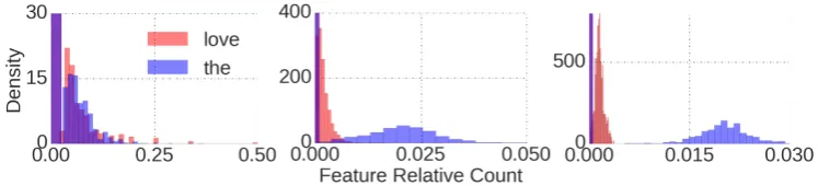
Figure 1 shows the distribution of two uni-grams, ‘the’ and ‘love’ at three levels of analy-sis. While both words have zero counts in most messages, ‘the’ starts to look Normal across

1_{Social Insights; Global social media research summary} 2017

users, and both words are approximately Normal at the county level. Methods performing optimally at the document level may suffer at the user or community level due to this shift in the distribu-tion of lexical features.2

In this paper, we ask a fundamental statistical question: How does the shift in unit-of-analysis from document-level to user-or-community level shift lexical distributions in social media?3 _The

central limit theorem suggests that count data is better approximated by a Normal distribution as one increases the number of events, or as one ag-gregates more features (e.g. combining words us-ing LDA topics or hand-built word sets). However, we do not know how far towards a Normal these new levels of analysis bring us.

Related work. The question we ask harks back to work from pioneers in corpus-based computational linguistics, including Shannon (1948) who suggested that probabilistic distribu-tions of ngrams could be used to solve a range of communications problems, and Mosteller and Wallace (1963) who found that a negative bino-mial distribution seemed to model unigram usage by authors of the Federalist Papers. Numerous works have since continued the tradition of ex-amining the distribution of lexical features. For example, McCallum et al. (1998) compares the results of probabilistic models based on multi-variate Bernoulli with those based on multinomial distributions for document classification. Jansche

2_{While the distribution of word frequencies (i.e. aZipfian} distribution) is often discussed in NLP, it is important to note that we are focused on the distribution of single features (e.g. words) over documents, users, or communities.

3_{While other sources of corpora can also be aggregated} to the user- or community-level (e.g. newswire, books), we believe the question of distributions is particularly important in social media because it often contains very short posts and a growing body of work in NLP for social science focuses on social media.

Figure 1: Histograms for unigrams “the” (a very frequent feature) and “love” (less frequent) at different levels of analysis: message, user, and community (from left to right). The bars at zero are cut-off at the message and user levels to increase readability of the remaining distribution.

(2003) extended this line of work, observing lex-ical count data often display an extra probability mass concentrated at zero and suggesting Zero-Inflated negative binomial distributions can cap-ture this phenomenon better and are easier to im-plement than alternatives such as overdispersed bi-nomial models. While these works are numerous, none, to the best of our knowledge, have focused on distributions across social media or at multiple levels of analysis.

Contributions. Our study is perhaps unconven-tional in modern computaunconven-tional linguistics due to the elementary nature of our contributions, focus-ing on understandfocus-ing the empirical distributions of lexical features in Twitter. First, we use zero-inflated kernel density estimated plots to show how distributions of different language features (words, LDA topics, and hand-curated word sets) vary with level of analysis (message, user, and county). Second, we quantify which distributions best describe the different feature types and anal-ysis levels of social media. Finally, we show the utility of such information, finding that us-ing the appropriate model for each feature type improves Naive Bayes classification results across three common social scientific tasks: sarcasm de-tection at the message-level, gender identification at the user-level, and political ideology classifica-tion at the community-level.

2 Methods

Examining data at three different levels of analy-sis and across three different lexical feature types (unigrams, data-driven topics, and manual lexica), we seek to (1) visually characterize distributions, (2) empirically test which distributions best fit the data, and (3) evaluate classification models utiliz-ing multiple distributions at each level. Unigrams underlie all data where as each level of analysis

and feature type represent a different degree of ag-gregation and covariance structure.

Data preparation. We start with a set of about two million Twitter posts and supplemental infor-mation about the users: their ID, county, and gen-der. The data was based on that ofVolkova et al.

(2013), who provide tweet ids and gender, and mapped to counties using the method ofSchwartz et al. (2013a). We limit our data to users who have used at least 1000 words and counties that have at least 30 users and a total word count of 5000. Applying these constraints, the final set of data consists of 1,639,750 tweets (representing the message-level) from 5,226 users in 420 different counties (representing the community-level).

We consider three lexical features that are commonly used in NLP for social science: 1-grams (the top 10,000 most common unigrams found with happierFunTokenizing social media tokenizer), 2000 LDA topics downloaded from

Schwartz et al.(2013b)), andlexica(64 categories from the linguistic inquiry and word count dictio-nary (Pennebaker et al.,2007)). Note that the fea-tures progress from most sparse (1grams) to least sparse (lexica).

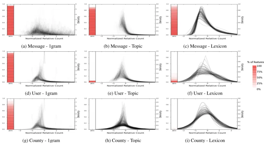
Distributions. Figure2shows the empirical dis-tributions of different lexical features at differ-ent levels of analysis. 500 features were sampled from the top 20,000 unigrams4_{, 2000 social}

me-dia LDA topics (Schwartz et al., 2013a), and all 64 categories from the LIWC lexica (Pennebaker et al., 2007). To encode the variables continu-ously we used relative frequencies for unigrams and lexica (count of word or category divided by count of all words), and probability of topics, cal-culated from the posterior probabilities from the LDA models. Each line in the kernel density plot

Figure 2:Kernel Density Estimate (KDE) plots showing the distribution of 500 random features at different levels of analysis. Each row represents a specific level of analysis (county, user, message) and each column represents a specific type of feature (Lexicon, Topic, Unigram). The bar on the left of each plot represents the percentage of observations that are zero for each feature where the shading represents the percent of features reaching the given threshold. As the bar gets darker it means more features out of 500 are zero in that percentage of individuals. The right portion of each plot is based on standardized relative frequencies of the variables (mean centered and divided by the standard deviation).

is semi-transparent such that an aggregate trend across multiple features will emerge darkest. As we move along a row ranging specific features (unigrams) to generic features (lexicon), the em-pirical distribution gradually changes from resem-bling a “power law” (or binomial distribution with low number of trials and probability of success) to something more “Normal”. Similar shifts are also observed as we move across levels of modeling.

We investigate whether the best-fitting distribu-tions vary across the three levels of analysis and three types of lexical features. We consider the following candidate distributions to see how well they fit each of these empirical distributions:

• Continuous Distributions: (a) Power-law,

(b), Log-normal and (c) Normal

• Discrete Distributions: (a) Bernoulli, (b) Multinomial, (c) Poisson, and (d) Zero In-flated Poisson

Since most of the distributions outlined above are standard distributions, we only briefly describe the zero-inflated variants which handle excess zero counts. Zero-inflated models explicitly model the idea that a distribution does not fully capture the mass at0in real world data. They assume that the

data is generated from two components. The first

component is governed by a Bernoulli distribution that generates excess zeros, while the second com-ponent generates counts, some of which also could be zero (Jansche,2003).

3 Evaluation

We evaluate the distributions we considered by first characterizing the goodness of fit at different levels of analyses and then by their predictive per-formance on social media prediction tasks, both of which we describe below.

3.1 Goodness of fit

Following the central limit theorem, we seek to de-termine across the range levels of analysis and fea-ture types, whether the distribution can be approx-imated by a Normal. Focusing just on the non-zero portions of data encoded as relative frequencies, we quantify the fit of each candidate distribution to the data.

Dist Message User County 1gram Topic Lex. 1gram Topic Lex. 1gram Topic Lex.

Power Law 71 10 0 4 0 0 7 0 0

Log-Normal 25 89 100 96 97 64 92 86 44

Normal 4 1 0 0 3 36 1 14 56

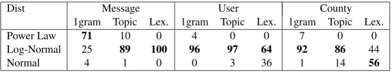
Table 1:Percentage of best-fitted distributions in each level of message, user, and county for different types of features such as “Lexicons”, “Topics”, and “1grams”. Note that the best-fitting distribution for each feature type is a function of the level of analysis.

is chosen as the ’best fit’ distribution. We repeat this100times and pick the most likely distribution

over all these100independent runs.

Results. Table 1 shows the percentage of fea-tures in each level that were best fit from an un-derlying distribution of Normal, Log-Normal, or Power Law. We see empirically that there is a trend toward Normal approximation moving from message to county level, as well as 1grams to lex-ica. In fact, a majority of lexica at the county-level were best approximated by a Normal distribution.

3.2 Predictive Power

In the previous section, we showed that the dis-tribution of lexical features depends on the scale of analysis considered (for example, the message level or the user level). Here, we demonstrate that predictive models which use these lexical fea-tures as co-variates can leverage this information to boost predictive performance. We consider three predictive tasks using a generative predictive model. The primary purpose of this evaluation is not to characterize the best distribution at a level or task, but to demonstrate that the choice of distribu-tion assumed when modeling features significantly affects the predictive performance.

Predictive Tasks : We consider the following common predictive tasks and also outline details of the datasets considered:

1. Sarcasm Detection (Message level): This task consists of determining whether tweets contain a sarcastic expression (Bamman and Smith,2015). The dataset consists of 16,833 messages with an average of 12 words per message.

2. Gender Identification (User level): This task involves determining the gender of the author utilizing a previously described Twit-ter dataset (Volkova et al.,2013). This dataset consists of 5,044 users each of which have

at least a 1,000 tokens as is standard in user-level analyses (Schwartz et al.,2013b).

3. Ideology Classification (Community level): We utilized county voting records from 2012 along with a dataset of tweets mapped to counties. This data consists of 2,175 counties with atleast 10,000 unigrams as is common in community level analyses (Eichstaedt et al.,

2015).

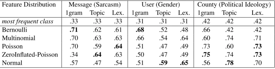
We consider a Naive Bayes classifier (a gener-ative model) which enables one to directly incor-porate the inferred feature distribution at a partic-ular level of analysis, the results of which we dis-cuss in Table 2. Variable encoding for the clas-sifiers varied from binary encoding of present or not (Bernoulli), to counts (Poisson, Zero-inflated Poisson), multivariate counts (Multinomial), and continuous relative frequencies (Normal). All dis-tributions have closed form MLE solutions ex-cept for Zero-Inflated Poisson, in which case we used LBFGS optimization to fit both of its param-eters (Head and Zerner,1985).

Results. We report macro F1-score for each of the underlying distributions in Table2. For each of the tasks, we used 80% of the data for

train-ing and evaluate on the held-out20%. We observe

con-Feature Distribution Message (Sarcasm) User (Gender) County (Political Ideology) 1gram Topic Lex. 1gram Topic Lex. 1gram Topic Lex.

most frequent class .33 .33 .33 .31 .31 .31 .42 .42 .42 Bernoulli .71 .62 .61 .68 .52 .48 .66 .42 .42 Multinomial .70 .63 .63 .66 .54 .64 .60 .74 .71

Poisson .70 .59 .64 .51 .47 .49 .73 .60 .73

ZeroInflated-Poisson .34 .64 .63 .50 .47 .49 .75 .74 .73

Normal .57 .47 .54 .51 .59 .65 .56 .78 .70

Table 2:F1-Score of Naive Bayes classifiers using various distributions and levels of analysis across tasks of sarcasm detec-tion, gender identificadetec-tion, and political ideology classification. Observe that predictive power is once again a function of the distribution family used to model feature distribution and depends on level of analysis.

sidered a function of level of analysis and feature-type considered and has a significant bearing on predictive performance.

4 Conclusion

While computational linguistics has a long his-tory of studying the distributions of lexical fea-tures, social media and social scientific studies have brought about a need to understand how these change at multiple levels of analyses. Here, we explored empirical distributions of different types of linguistic features (unigrams, topics, lexica) in three different levels of analysis in Twitter data (message, user, and community). To show which distribution can better describe features of differ-ent levels, we approached the problem in three dif-ferent ways: (1) visualization of empirical distri-butions, (2) goodness-of-fit comparisons, and (3) for predictive tasks.

We showed that the best-fit distribution depends on feature-type (i.e. unigram versus lexica) and the level of analysis (i.e. message-, user-, or community-level). Following the central limit the-orem, all user-level features were predominantly Log-normal, while a power law best fit unigrams at the message level and a Normal distribution best approximated lexica at the community level. Finally, we demonstrated that predictive perfor-mance can also vary considerably by the level of analysis and feature-type, following a similar trend from Bernoulli distributions at the message-level to Poisson or Normal at the community-message-level. Our results underscore the significance of the level of analysis for the ever-growing focus in NLP on social scientific problems which seek to not only better model words and documents but also the people and communities generating them.

Acknowledgements

This work was supported in part by the Templeton Religion Trust, Grant TRT-0048.

References

David Bamman and Noah A Smith. 2015. Contextu-alized sarcasm detection on twitter. InProceedings to the International Conference on Web-blogs and Social Media. pages 574–577.

Glen Coppersmith, Mark Dredze, and Craig Harman. 2014. Quantifying mental health signals in twitter. In Proceedings of the ACL workshop on Computa-tional Linguistics and Clinical Psychology.

Johannes C Eichstaedt, H Andrew Schwartz, Mar-garet L Kern, Gregory Park, Darwin R Labarthe, Raina M Merchant, Sneha Jha, Megha Agrawal, Lukasz A Dziurzynski, Maarten Sap, et al. 2015. Psychological language on twitter predicts county-level heart disease mortality. Psychological Science

1:11.

Lucie Flekova, Jordan Carpenter, Salvatore Giorgi, Lyle Ungar, and Daniel Preoctiuc-Pietro. 2016. An-alyzing Biases in Human Perception of User Age and Gender from Text. InProceedings of the 54th annual meeting of the Association for Computa-tional Linguistics. ACL.

John D Head and Michael C Zerner. 1985. A broyden-fletchergoldfarbshanno optimization procedure for molecular geometries. Chemical physics letters

122(3):264–270.

Martin Jansche. 2003. Parametric models of linguistic count data. InProceedings of the 41st Annual Meet-ing on Association for Computational LMeet-inguistics- Linguistics-Volume 1. Association for Computational Linguis-tics, pages 288–295.

Andrew McCallum, Kamal Nigam, et al. 1998. A com-parison of event models for naive bayes text classi-fication. InAAAI-98 workshop on learning for text categorization. Citeseer, volume 752, pages 41–48.

Frederick Mosteller and David L Wallace. 1963. In-ference in an authorship problem: A comparative study of discrimination methods applied to the au-thorship of the disputed federalist papers.Journal of the American Statistical Association 58(302):275– 309.

James W Pennebaker, Roger J Booth, and Martha E Francis. 2007. Liwc2007: Linguistic inquiry and word count. Austin, Texas: LIWC.net.

Ruchita Sarawgi, Kailash Gajulapalli, and Yejin Choi. 2011. Gender attribution: tracing stylometric evi-dence beyond topic and genre. In Proceedings of the Fifteenth Conference on Computational Natural Language Learning. Association for Computational Linguistics, pages 78–86.

H Andrew Schwartz, Johannes C Eichstaedt, Mar-garet L Kern, Lukasz Dziurzynski, Richard E Lucas, Megha Agrawal, Gregory J Park, Shrinidhi K Lak-shmikanth, Sneha Jha, Martin EP Seligman, et al. 2013a. Characterizing geographic variation in well-being using tweets. InProceedings of the 7th Inter-national AAAI Conference on Web and Social Me-dia. ICWSM.

H Andrew Schwartz, Johannes C Eichstaedt, Mar-garet L Kern, Lukasz Dziurzynski, Stephanie M Ra-mones, Megha Agrawal, Achal Shah, Michal Kosin-ski, David Stillwell, Martin EP Seligman, et al. 2013b. Personality, gender, and age in the language of social media: The open-vocabulary approach.

PloS one8(9):e73791.

H Andrew Schwartz and Lyle H Ungar. 2015. Data-driven content analysis of social media a systematic overview of automated methods. The ANNALS of the American Academy of Political and Social Sci-ence659(1):78–94.

Claude E Shannon. 1948. A mathematical theory of communication, bell system technical journal 27: 379-423 and 623–656. Mathematical Reviews (MathSciNet): MR10, 133e.