Munich Personal RePEc Archive
A folk theorem in infinitely repeated
prisoner’s dilemma with small
observation cost
Hino, Yoshifumi
Vietnam-Japan University
10 December 2018
Online at
https://mpra.ub.uni-muenchen.de/96010/
A folk theorem in infinitely repeated prisoner’s
dilemma with small observation cost
∗
Yoshifumi Hino
†This version: September 13, 2019
Abstract
We consider an infinitely repeated prisoner’s dilemma under costly monitoring. If a player observes his opponent, then he pays an observa-tion cost and knows the acobserva-tion chosen by his opponent. If a player does not observe his opponent, he cannot obtain any information about his opponent’s action. Furthermore, no player can statistically identify the observational decision of his opponent. We prove efficiency without any signals. Then, we extend the idea with a public randomization device and we present a folk theorem for a sufficiently small observation cost when players are sufficiently patient.
Keywords Costly observation; Efficiency; Folk theorem; Prisoner’s dilemma
JEL Classification: C72; C73; D82
1
Introduction
A now standard insight in the theory of repeated games is that repetition enables players to obtain collusive and efficient outcomes in a repeated game. However, a common and important assumption behind such results is that the players in the repeated game can monitor each other’s past behavior without any cost. We analyze an infinitely repeated prisoner’s dilemma game where each player can only observe or monitor his opponent’s previous action at a (small) cost and a player’s monitoring decision is unobservable to his opponent. We establish an approximate efficient result together with a corresponding approximate folk theorem.
∗This research did not receive any specific grant from funding agencies in the public,
commercial, or not-for-profit sectors.
†Business Administration Program, Vietnam–Japan University, Luu Huu Phuoc Street,
My Dinh 1 Ward, Nam Tu Liem District, Hanoi, 129060, Vietnam Tel: +84 24 7306 6001
In our model, we consider costly monitoring as a monitoring structure. Each player chooses his action and makes an observational decision. If a player chooses to observe his opponent, then he can observe the action chosen by the opponent. The observational decision itself is unobservable. The player cannot obtain any information about his opponent in that period if he chooses not to observe that player.
Furthermore, no player can statistically identify the observational decision of his opponent. That is, our monitoring structure is neither almost-public private monitoring (H¨orner and Olszewski (2009); Mailath and Morris (2002, 2006); Mailath and Olszewski (2011)), nor almost perfect private monitoring (Bhaskar and Obara (2002); Chen (2010); Ely and V¨alim¨aki (2002); Ely et al. (2005); H¨orner and Olszewski (2006); Sekiguchi (1997); Piccione (2002); Yamamoto (2007, 2009))
We present two results. First, we show that the symmetric Pareto efficient payoff vector can be approximated by a sequential equilibrium without any signals under some assumptions regarding the payoff matrix when players are patient and the observation cost is small (efficiency). The second result is a type of folk theorem. We introduce a public randomization device. The public randomization device is realized at the end of each stage game, and players see the public randomization device without any cost. We present a folk theorem with a public randomization device under some assumptions regarding the payoff matrix when players are patient and the observation cost is small. The first result shows that cooperation is possible without any signals or communication in the venture company example. The second result implies that companies need a coordination device to achieve an asymmetric cooperation in the venture company example.
The nature of our strategy is similar to thekeep-them-guessing strategiesin Chen (2010). In our strategy, each player i chooses Ci with certainty at the
cooperation state, but randomizes the observational decision. Depending on the observation result, players change their actions from the next period. If the player plays Ci and observesCj, he remains in a cooperation state. However,
in other cases (for example, the player does not observe his opponent), playeri
moves out of the cooperation state and chooses Di. From the perspective of
player j, playeri plays the game as if he randomizesCi andDi, even though
playerichooses pure actions in each state. Such randomized observations create uncertainty about the opponents’ state in each period and give an incentive to observe.
As with Chen (2010), our analysis is tractable. By construction, the only concern of each player at each period is whether his opponent is in the cooper-ation state. It is sufficient to keep track of this belief, which is the probability that the opponent is in the cooperation state.
before we define our model in Section 3. Our efficiency result shows that players can construct a cooperative relationship without any randomization device.
Another contribution of the paper is a new approach to the construction of a sequential equilibrium. We consider randomization of monitoring, whereas previous studies confine their attention to randomization of actions. In most cases, the observational decision is supposed to be unobservable in costly mon-itoring models. Therefore, even if a player observes his opponent, he cannot know whether the opponent observes him. If the continuation strategy of the opponent depends on the observational decision in the previous period, the op-ponent might randomize actions from the perspective of the player, even though the opponent chooses pure actions in each history. This new approach enables us to construct a nontrivial sequential equilibrium.
The rest of this paper is organized as follows. In Section 2, we discuss pre-vious studies, and in Section 2.1, we focus on some prepre-vious literature and ex-plain some difficulties in constructing a cooperative relationship in an infinitely repeated prisoner’s dilemma under costly monitoring. Section 3 introduces a re-peated prisoner’s dilemma model with costly monitoring. We present our main idea and results in Section 4, including an efficiency result with a small obser-vation cost. We extend our main idea with a public randomization device and present a folk theorem in Section 5. Section 6 provides concluding remarks.
2
Literature Review
We only review previous studies on repeated games with costly monitoring. One of the biggest difficulties in costly monitoring is monitoring the moni-toring activity of opponents, because observational behavior under costly mon-itoring is often assumed to be unobservable. Each player has to check this un-observable monitoring behavior to motivate the other player to observe. Some previous studies circumvent the difficulty by assuming that the observational decision is observable. Kandori and Obara (2004); Lehrer and Solan (2018) assume that players can observe other players’ observational decisions.
Next approach is communication. Ben-Porath and Kahneman (2003) an-alyze an information acquisition model with communication. They show that players can share their information through explicit communication, and present a folk theorem for any level of observation cost. Ben-Porath and Kahneman (2003) consider randomizing actions on the equilibrium path. In their strategy, players report their observations to each other. Then, each player can check whether the other player observes him by the reports. Therefore, players can check the observation activities of other players.
Another approach is introduction of nonpublic randomization device. The nonpublic randomization device enables players randomize actions even though they are certain that both players are in the cooperation state. Hino (2019) shows that if nonpublic randomization device is available before players choose their actions and observational decisions, then players can achieve an efficiency result.
If these assumptions do not hold, that is, if no costless information is avail-able, then cooperation is difficult. Two other papers present folk theorems with-out costless information. Flesch and Perea (2009) consider monitoring structures similar to our structure. In their model, players can purchase the information about the actions taken in the past if the players incur an additional cost. That is, some organization keeps track of all the sequence of the action profiles, and each player can purchase the information from the organization. Flesch and Perea (2009) present a folk theorem for an arbitrary observation cost. Miyagawa et al. (2003) consider less stringent models. They assume that no organization keeps track of all the sequence of the action profiles for players. Players can observe the opponent’s action in the current period, and cannot purchase the information about the actions in the past. Therefore, if a player wants to keep track of actions chosen by the opponent, he has to pay observation cost every period. This monitoring structure is the same as the one in the current paper. Miyagawa et al. (2003) present a folk theorem with a small observation cost.
The above two studies, Flesch and Perea (2009) and Miyagawa et al. (2003), consider implicit communication through mixed actions. To use implicit com-munication by mixed actions, the above two papers need more than two actions for each player. This means that their approach cannot be applied to infinitely repeated prisoner’s dilemma under costly . We discuss their implicit commu-nication in Miyagawa et al. (2003); Flesch and Perea (2009) in Section 2.1 in more detail.
It is an open question whether players can achieve an efficiency result and a folk theorem in 2-action games, even though the monitoring cost is sufficiently small. We show an efficiency result without any randomization device using a grim trigger strategy and mixed monitoring rather than mixed actions when observation cost is small. Since we use a grim trigger strategy, players have no incentive to observe the opponent once after the punishment has started. In addition, in our strategy, players choose different actions when they are in the cooperation state and when they are in another state. Therefore, the observation
in the current period gives player i enough information to check whether the
2.1
Cooperation failure in the prisoner’s dilemma
(Miya-gawa et al. (2003))
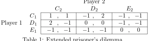
Consider the bilateral trade game with moral hazard in Bhaskar and van Damme (2002) simplified by Miyagawa et al. (2003).
Player 2
C2 D2 E2
Player 1
C1 1 , 1 −1 , 2 −1 , −1
D1 2 , −1 0 , 0 −1 , −1
[image:6.612.185.435.190.259.2]E1 −1 , −1 −1 , −1 0 , 0 Table 1: Extended prisoner’s dilemma
Players choose whether he observes the opponent or not at the same time with his action choice. Miyagawa et al. (2003) consider the following keep-them-guessing grim trigger strategies to approximate payoff vector (1,1). There are three states: cooperation, punishment, and defection. In the defection state,
both players choose Ei, and the state remains the same. In the punishment
state, both players chooseEi for some periods, and then the state moves back
to a cooperation state. In both the punishment state and the defection state, the players do not observe their opponent. In the cooperation state, each player choosesCiwith sufficiently high probability and choosesDi with the remaining
probability. Players observe their opponent in the cooperation state. If players observe (C1, C2) or (D1, D2), the state remains the same. The state moves to the defection state if player i chooses Ei or observes Ej. When (C1, D2) or
(D1, C2) is realized, the state moves to the punishment state.
Players have an incentive to observe their opponent because their opponent randomizes actions Cj and Dj in the cooperation state. If a player does not
observe their opponent, the player cannot know the state of the opponent in the next period. If the state of the opponent is the cooperation state, then actionEiis a suboptimal action because the opponent never chooses actionEj.
That is, choosing actionEi has some opportunity cost because the state of the
opponent is the cooperation state with a high probability. However, if the state of the opponent is the defection state, then actionEiis a unique optimal action.
Choosing actionsCi or Di also has opportunity costs because the state of the
opponent is the punishment state with a positive probability. To avoid these opportunity costs, players have an incentive to observe.
These ideas do not hold in two-action games. Let us consider the prisoner’s
dilemma as an example. If players randomize Ci and Di in the cooperation
state, then their best response action includes actionDi at any history. As a
result, choosing Di and not observe player j every period is one of the best
response strategy. The strategy fails to give players monitoring incentive. I consider the following strategy. In the cooperation state, playeri chooses
action Ci with probability one, but randomizes observational decision. Only
if playeri choosesCi and observesCj, player ican remain in the cooperation
Using this strategy, we show an efficiency result without any randomization device, and we extend it with public randomization device and present a folk theorem.
The reason why our strategy works in a two-action game is that the strat-egy prescribes different actions based on the observation result. The stratstrat-egy prescribes action Ci (resp., Di) when player i observes action oi = Ci (resp.,
oi=Dj). Hence, player idoes not randomize actionsCi andDi in each period
except for the initial period, and the above-mentioned problem does not occur. The above-mentioned problem does not happen in the initial because there is no previous period of the initial period and playeridoes not observe the opponent in the previous period.
However, it causes another problem related to the monitoring incentive. As playerjdoes not randomize his action, playerican easily guess playerj’s action through past observation. For example, if playerichooses Ci and observedCj
in the previous period, playerican guess that playerj’s action will beCj. Then,
playeriloses the monitoring incentive again.
Our strategy can overcome this difficulty as well. Since player j randomize his observational decision in the cooperation state and it is unobservable, playeri
in the cooperation state cannot know whether playerjobserved playerior not. Suppose that playerichoosesCiin the previous period. Then, if playerjchooses
Cj and observed playeriin the previous period, playerj is in the cooperation
state in the current period and chooses Cj. Otherwise, player j chooses Dj
in the current period. Therefore, from the viewpoint of player i, it looks as if playerj randomizes actions Cj andDj, which gives playeri an incentive to
observe. This is why player i has an incentive to observe player j given our
strategy.
3
Model
The base game is a symmetric prisoner’s dilemma. Each player i (i = 1,2)
chooses an action,CiorDi. LetAi≡ {Ci, Di}be the set of actions for playeri.
Given an action profile (a1, a2), the base game payoff for playeri,ui(a1, a2), is
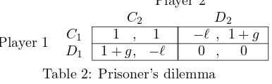
displayed in Table 2.
Player 2
C2 D2
Player 1 C1 1 , 1 −ℓ , 1 +g
[image:7.612.214.407.534.594.2]D1 1 +g, −ℓ 0 , 0 Table 2: Prisoner’s dilemma
We make the usual assumptions about the above payoff matrix.
Assumption 1. (i)g >0 andℓ >0; (ii)g−ℓ <1.
The first condition implies that actionCi is dominated by action Di for each
Assumption 2. g−ℓ >0.
Assumption 2 is the same as Assumption 1 in Chen (2010).
The stage game is of simultaneous form. Each playerichooses an actionai
and the observational decision simultaneously. Let mi represent the
observa-tional decision for playeri. LetMi≡ {0,1}be the set of observational decisions
for playeri, where mi = 1 represents “to observe the opponent,” and mi = 0
represents “not to observe the opponent.” If playeriobserves the opponent, he incurs an observation costλ >0, and receives complete information about the
action chosen by the opponent at the end of the stage game. If player idoes
not observe the opponent, he does not incur any observation cost and obtains no information about his opponent’s action. We assume that the observational decision for a player is unobservable.
A stage behavior for playeriis the pair of base game actionsai for playeri
and observational decisionmi for playeriand is denoted by bi = (ai, mi). An
outcome of the stage game is the pairb1andb2. LetBi≡Ai×Mibe the set of
stage-behaviors for playeri, and letB≡B1×B2be the set of outcomes of the stage game. Given an outcomeb∈B, the stage game payoffπi(b) for playeri
is given by
πi(b)≡ui(a1, a2)−miλ.
For any observation costλ >0, the stage game has a unique stage game Nash equilibrium outcome,b∗= ((D1,0),(D2,0)).
Letδ∈(0,1) be a common discount factor. Players maximize their expected average discounted stage game payoffs. Given a sequence of outcomes of the stage games (bt)∞
t=1, playeri’s average discounted stage game payoff is given by
(1−δ) ∞
∑
t=1
δt−1πi(bt).
During the repeated game, players does not receive any free signals regarding player actions (no free signal). It implies that a player receives no information about the action chosen by his opponent when he does not observe the opponent. This implies that no player receives the base game payoffs in the course of play. As in Miyagawa et al. (2003), we interpret the discount factor as the probability with which the repeated game continues, and it is assumed that each player receives the sum of the payoffs when the repeated game ends. Then, the assumption of no free signals regarding actions is less problematic.
Let oi ∈ Aj ∪ {ϕi} be an observation result for player i. Observation
re-sultoi=aj∈Aj implies that playeri chose observational decisionmi= 1 and
observedaj. Observation resultoi=ϕi implies that playerichosemi= 0, that
is, he obtained no information about the action chosen by the opponent. Letht
i be the (private) history of player iat the beginning of periodt≥2:
ht
i = (aki, oki) t−1
k=1. This history is a sequence of his own actions and observation
results up to periodt−1. We omit the observational decisions fromht
i because
observation resultok
denote the set of all the histories for playeri at the beginning of periodt≥1,
whereH1
i is an arbitrary singleton set.
A (behavior) strategy for playeriin the repeated game is a function of the history of playeri to his (mixed) stage behavior.
The beliefψt
i of playeriin periodtis a function of the historyhti of playeri
in periodt obtained from a probability distribution over the set of histories for playerj in periodt. Letψi≡(ψit)∞t=1be a belief for playeri, andψ= (ψ1, ψ2)
denote a system of beliefs.
A strategy profile σ is a pair of strategies σ1 and σ2. Given a strategy profile σ, a sequence of completely mixed behavior strategy profiles (σn)∞
n=1
that converges toσis called atremble. Each completely mixed behavior strategy profileσn induces a unique system of beliefsψn.
The solution concept is a sequential equilibrium. We say that a system of beliefsψ is consistent withσ if a tremble (σn)∞
n=1 exists such that the
corre-sponding sequence of system of beliefs (ψn)∞
n=1converges toψ. Given the system
of beliefs ψ, strategy profile σis sequentially rational if, for each player i, the continuation strategy from each history is optimal given his belief of the history and the opponent’s strategy. It is defined that a strategy profileσis asequential equilibriumif a consistent system of beliefsψfor whichσis sequentially rational exists.
4
No public randomization
In this section, we show our efficiency result without any randomization device. The following proposition shows that the symmetric efficient outcome is approx-imated by a sequential equilibrium if the observation cost λ is small and the discount factorδis moderately low.
Proposition 1. Suppose that Assumptions 1 and 2 are satisfied. For anyε >0, there exist δ ∈ (1+gg,1), δ ∈ (δ,1), and λ > 0 such that for any discount factorδ∈[δ, δ]and for any observation costλ∈(0, λ), there exists a symmetric sequential equilibrium whose payoff vector (v∗
1, v2∗)satisfiesv∗i ≥1−ε for each
i= 1,2.
Proof. See Appendix A.
An illustration
While the proof in Appendix A provides the detailed construction of an equi-librium that approximates the Pareto-efficient payoff vector, we here present its main idea.
Let us consider the following four-state automaton: initial stateω1
i,
cooper-ation state (ωt
i)∞t=2, transition stateωiE, and defection state ωDi . In the initial
stateω1
i, playerirandomizes three stage-behaviors: (Ci,1), (Ci,0), and (Di,0).
stateωt
i(t≥2), playeri choosesCi and randomizes the observational decision.
Playerichooses (Ci,1) with sufficiently high probability. In the transition state
and defection stateωD
i , playerichooses (Di,0).
The state transition is described in Figure 1.
ω1
i ω2i ω3i ωit
(a1
i, o1i) = (Ci, Cj)
. . .
(at
i, oti) = (Ci, Cj)
. . .
ωE i
(ai, oi) = (Ci, ϕi)
oi=ϕi
ωD i
ai =Di
or
oi =Dj
ai =Di
or
oi =Dj
If (at
i, oti) = (Ci, Cj)
atωE
i in periodt,
the state in pe-riodt+ 1 isωt+1
i
Figure 1: The state-transition rule
That is, a player remains in the cooperation state only when he chooses Ci
and observes Cj. Player i moves to the defection state if he chooses Di or
observesDj. If playeridoes not observe his opponent in the cooperation state,
he moves to the transition state. Although, the stage-behavior in the transition state is the same as that in the defection state, the transition function is not.
Player i moves back to the cooperation state from the transition state if he
observes (Ci, Cj), which is the event off the equilibrium path. Let strategyσ∗
be the strategy above.
Another property of this strategy is that players never randomize their ac-tions in the cooperation state, whereas players randomize their observational decisions in the cooperation state. As a result, the player looks as if he ran-domizes actions from the viewpoint of his opponent although he chooses pure
actions in each state. Furthermore, we show in the appendix that player i
strictly prefers action Ci in the cooperation state although he strictly prefers
actionDi in the defection state. This creates a monitoring incentive in order to
know which action is optimal.
Let us consider sequential rationality in each state. First, we consider the defection state. A sufficient condition for sequential rationality in the defection state is that playeri is certain that the state of the opponent is the transition or defection state. It implies that playeriis sure that playerj choosesDj and
never observes playeri. Hence, playeridoes not have an incentive to chooseCi
ormi= 1 in the defection state on the equilibrium path.
The defection state occurs only when playerichooses Di or observedDj in
The defection state might be realized off the equilibrium path. Then, it is not obvious whether this sufficient condition holds off the equilibrium path or not. Let us consider the following history in period 3. Playerichoosesai=Di
andmi = 0 in period 1, and he chooses ai =Ci and observes Cj in period 2.
We can consider the following history. Playerj choosesaj=Cj andmj = 0 in
period 1, and he choosesaj =Cj (by mistakes) and observes Cj (by mistake)
in period 2. Then, playerj is in the cooperation state in period 3.
To obtain the desired belief, we consider the same belief as Miyagawa et al. (2008). That is, we consider a sequence of behavioral strategy profiles (ˆσn)∞
n=1
such that each strategy profile attaches a positive probability to every move, but puts far smaller weights on the trembles with respect to the observational decisions compared with those with respect to actions1. These trembles induce
a consistent system of beliefs that playeriat any defection state is sure that the state of their opponent is the defection state. It ensures the sufficient condition. Let us discuss sequential rationality in the cooperation state. First of all, we consider how to find the sequence of randomization probabilities of stage-behaviors. We define the sequence as follows. We fix small probability of choos-ingDjin the initial probability. Then, we can derive the payoff for playeriwhen
playerichooseDiin the initial period based on probability ofDj. Playerimust
be indifferent betweenCi andDi in the initial period. The continuation payoff
from the cooperation state in period 2 is the continuation payoff when playeri
chooses Ci and does not observe the opponent in period 2. It is the function
of the probabilities of choosingDj and of monitoring in the initial period. We
choose monitoring probability in the initial period to make playeri indifferent
between Ci and Di. The similar argument holds in period 2 onwards. The
continuation payoff from the cooperation state in period t ≥ 3 is the
contin-uation payoff when playeri chooses Ci and does not observe the opponent in
periodt. It is the function of the probabilities of monitoring in the previous and current period. In period 2, we know the monitoring probability in the ini-tial period. Therefore, we choose the monitoring probability in the period 2 so that playeriis indifferent between observing and not observing in period 2. In periodt(≥3), we know the monitoring probability in the previous period, and we choose the monitoring probability in periodt so that player iis indifferent between observing and not observing in periodt.
Then, the sequential rationality in the initial and cooperation states is satis-fied as follows. In the initial state, playeriis indifferent betweenCiandDi, and
is indifferent between observing and not observing because of the randomization probability ofDi and the definition of the monitoring probability in the initial
state. It is suboptimal that choosing Di but observing the opponent because
playeri is certain that the opponent is no longer in the cooperation state irre-spective his observational result. In periodt≥2, playeriis indifferent between observing and not observing by the selection of the monitoring probability of player j in the current period. It is also suboptimal to choose Di and observe
the opponent as the same as in the initial period. Furthermore, this definition
ensures that playeri strictly prefers action Ci to Di in the cooperation state.
Suppose that player i weakly prefers actionDi in the next cooperation state.
Then, choosing actionDiis the best response action irrespective of his
observa-tion result. This means that playeristrictly prefersmi= 0 because he can save
the observation cost by choosing (Ci,0) in the current period and (Di,1) in the
next period. Hence, playeri strictly prefers actionCi in the next cooperation
state after he choosesCi and observes Cj in the cooperation state. Therefore,
sequential rationality is satisfied in the cooperation state.
Next, let us consider the transition state. We show why player i prefers
actionDi in the transition state. In the transition state, there are two types
of situations. Situation A is where player i is in the cooperation state if he
observed his opponent in the previous period. Situation B is where player i
is in a defection state if he observed his opponent in the previous period. Of course, playericannot distinguish between these two situations because he did not observe his opponent. To understand sequential rationality in the transition state, let us assume that the monitoring cost is almost zero. This means that the deviation payoff to (Di,0) in the cooperation state is sufficiently close to
the continuation payoff from the cooperation state. Otherwise, playeristrictly prefers to observe in the cooperation state to avoid choosing actionDi in
situa-tionA. Therefore, playeriis almost indifferent between choosingCi andDi in
situation A, whereas playeri strictly prefers actionDi in situation B. Hence,
playeristrictly prefers actionDi when the observation cost is sufficiently small
because both situations are realized with a positive probability.
Third, let us consider the initial state. The indifference condition betweenCi
andDi is ensured by the randomization probability between (Ci,1) and (Ci,0)
in the initial state. If the monitoring probability in the cooperation state is high enough, then playeriis willing to choose actionCi. The indifference condition
between (Ci,1) and (Ci,0) in the initial state is ensured by the randomization
probability between (Ci,1) and (Ci,0) in the cooperation state in period 2.
There is no incentive to choose (Di,1) because the state of the opponent in the
next period is not the cooperation state for sure, irrespective of the observation. Lastly, let us consider the payoff. It is obvious that the equilibrium payoff vector is close to 1 if the probabilities of (Ci,1) in the initial state and
cooper-ation state are close to 1 and the observcooper-ation cost is close to 0. In Appendix A, we show that the equilibrium payoff vector is close to 1 when the discount factor is close to 1+gg. Another remaining issue is whether our strategy is well-defined, which is shown by solving a difference equation of monitoring constraints in Appendix A when Assumption 2 is satisfied.
We extend Proposition 1 using Lemma 1.
Lemma 1. Fix any payoff vector v and any ε > 0. Suppose that there exist
δ∈(1+gg,1),δ∈(δ,1)such that for any discount factorδ∈[δ, δ], there exists a sequential equilibrium whose payoff vector(v∗
1, v2∗)satisfies|vi∗−vi| ≤εfor each
i= 1,2. Then, there existδ∗∈(g/1 +g,1)such that for any discount factorδ∈
[δ∗,1), there exists a sequential equilibrium whose payoff vector(v∗
1, v2∗)satisfies
|v∗
Proof of Lemma 1 . We use the technique of Lemma 2 in Ellison (1994). We define δ∗ ≡ δ/δ, and choose any discount factorδ ∈(δ∗,1). Then, we choose some integer n∗ that satisfies δn∗
∈ [δ, δ]. Then there exists a strategy σ′ whose payoff vector is (v∗
1, v2∗) given δn
∗
. We divide the repeated game into
n∗ distinct repeated games. The first repeated game is played in period 1,
n∗+ 1, 2n∗ + 1. . ., the second repeated game is played in period 2, n∗+ 1, 2n∗+ 2. . ., and so on. Each repeated game can be regarded as a repeated game with discount factorδn∗
. Let us consider the following strategyσL1. In the 1st
game, players follow strategyσ′. In the 2nd game, players follow strategyσ′. In then(n≤n∗)th game, players follow strategyσ′. Then, strategyσL1 will be a
sequential equilibrium. This is because strategyσ′ is a sequential equilibrium in each game. As the equilibrium payoff vector in each game satisfies|v∗
i −vi| ≤ε
for eachi= 1,2, the equilibrium payoff of strategyσL1also satisfies|v∗
i−vi| ≤ε
for eachi= 1,2.
We obtain efficiency for a sufficiently high discount factor.
Proposition 2. Suppose that the base game satisfies Assumptions 1 and 2. For any ε > 0, there exist δ∗ ∈ (0,1) and λ > 0 such that for any discount factorδ∈(δ∗,1)and anyλ∈(0, λ), there exists a sequential equilibrium whose payoff vector(v∗
1, v2∗) satisfiesvi∗≥1−εfor each i= 1,2.
Proof of Proposition 2 . Apply Lemma 1 to Proposition 1.
Remark 1. Proposition 2 shows monotonicity of efficiency on the discount factor. If efficiency holds givenε, observation costλand discount factorδ, then efficiency holds given a sufficiently large discount factorδ′ > δ.
Lastly, let us consider what happens if Assumption 2 is not satisfied. Letβ1
be the probability that playerichoosesai=Di in the first period. Letβt+1 be
the probability that playerichoosesmi= 0 in the cooperation stateωti. Then,
the following proposition holds.
Proposition 3. Suppose that Assumption 1 is satisfied, but 2 is not satisfied. Then,(βt)∞t=1 is not well defined for a small observation cost λ.
Proof of Proposition 3 . See Appendix C.
Proposition 3 implies that our strategy is not well-defined when 2 is not satisfied. Let us explain Proposition 3. A relationship betweenβt and βt+1 is
determined by the monitoring incentive and ℓ
g. We show that the absolute value
ofβtgoes to infinity ast goes to infinity when gℓ >1.
Let us derive the relationship. If player i chooses Ci and observes Cj in
stateωti−1, his continuation payoff from periodt is given by
On the other hand, if player i chooses Ci but does not observe player j, his
continuation payoff from periodtis
(1−δ)(1−βt)(1 +g).
Therefore, only when the following equation holds, playeriis indifferent between
mi= 0 andmi= 1 in state ωit−1.
λ δ(1−βt−1)
=−g+βt(g−ℓ) +δ(1−βt)(1−βt+1)(1 +g). (1)
Rewards for choosingmi= 1 comes from two parts: −g+βt(g−ℓ) and δ(1−
βt)(1−βt+1)(1 +g) in (1). Reward δ(1−βt)(1−βt+1)(1 +g) implies that
whenβtis too small (resp., large),βt+1must be large (resp., small) in order to
keep the right-hand side in (1) unchanged. Reward−g+βt(g−ℓ) implies that
wheng−ℓ >0 (resp.,g−ℓ <0), an increase inβtstrengthens (resp., weakens)
the monitoring incentive. This is because increase in βt implies decrease of
(1−βt)gand makes choosingDi in the next period less attractive. Increase in
βt also implies decrease of−βtℓ and makes choosingCi in the next period less
attractive. Therefore, whether larger βt strengthens the monitoring incentives
or not depends on whether Assumption 2 holds or not.
Assume that Assumption 2 holds, then these two rewards has opposite effect. Suppose thatβtis high. Then, the rewardδ(1−βt)(1−βt+1)(1 +g) prescribes
smallerβt+1 to maintain the monitoring incentive. On the other hand, reward
−g+βt(g−ℓ) strengthens the monitoring incentive and prescribes higherβt+1
in order to reduceδ(1−βt)(1−βt+1) and to weaken the monitoring incentive.
On the other hands, if Assumption 2 does not hold, then these two rewards have the same effect. Given high βt, the reward δ(1−βt)(1−βt+1)(1 +g)
prescribes smaller βt+1 to maintain the monitoring incentive. Reward −g +
βt(g−ℓ) weakens the monitoring incentive and prescribes smallerβt+1in order
to strengthen the monitoring incentive. As a result, the sequence (βt)∞t=1 will
be a divergent sequence.
Let us show this fact by an approximation. Let define ε′ ≡ δ− g
1+g and
assume thatε′ is sufficiently small. Then, assuming ε′, β
t, andβt+1 are small,
andλis sufficiently small compared to ε′, we can ignoreλ, β
t·βt+1, ε′βt and
ε′β
t+1. Then, we obtain
0 =−βtℓ+ (1 +g)ε′−βt+1g
or,
βt+1−
1 +g g+ℓε
′ =−ℓ
g
(
βt−
1 +g g+ℓε
′
)
(2)
The above equation (2) shows the relationship betweenβtandβt+1.
The ratio ℓ
g determines how largeβt+1 must be in order to satisfy the
(i.e., ℓ
g >1), the absolute value of βt+2−
1+g g+ℓε
′ must be larger than the
abso-lute value of βt+1− 1+g+gℓε′. As a result, the absolute value of βt−1+g+gℓε′ goes
to infinity astgoes to infinity. More precise calculation without approximation can be found in Appendix C.
Remark 2. Let us refer toσ∗in the proof of Proposition 1 andσL1in Lemma 1
as keep-them-monitoring grim trigger strategy. Proposition 1 and Proposition 3 shows a sufficient and necessary condition for keep-them-monitoring grim trigger strategy. A keep-them-monitoring grim trigger strategy is a sequential equilib-rium for a sufficiently large discount factor and a sufficiently small observation cost if and only if Assumption 2 is satisfied.
5
Public randomization
In this section, we assume the public randomization device is available at the end of each stage game. The distribution of the public signal is independent of the action profile chosen. Public signalxis uniformly distributed over [0,1) and each player observes the public signal without any cost.
The purpose of this section is to prove a folk theorem. To prove Theorem 1 (folk theorem), we present the following proposition first.
Proposition 4. Suppose that a public randomization device is available, and the base game satisfies Assumptions 1 and 2. For any ε > 0, there exist δ ∈
(
g
1+g,1
)
,δ∈(δ,1), and λ >0 such that for any discount factor δ∈[δ, δ] and for any observation cost λ∈(0, λ), there exists a sequential equilibrium whose payoff vector(v∗
1, v2∗) satisfiesv1∗= 0andv2∗≥ 1+1+g+ℓℓ−ε.
Proof of Proposition 4 . See Appendix D.
An illustration
Here we explain our strategy and why we need a public randomization device for our result.
In our strategy, the players play (C1, D2) in the first period and only player 2 observe, and then play the strategy in the proof of Proposition 1 from period 2 onward. Applying the strategy in Section 4, let us consider the following
strat-egy. At the initial state, player 1 randomizes actions C1 and D1, whereas
player 2 choosesD2. Player 2 randomly observes player 1. The state transition depends on public randomization. If realizedxis greater than ˆxin the initial state, the remains the same. If realized xis not greater than ˆx in the initial state, the state transition depends on the stage-behaviors. If player 1 playsD1
strategy is similar to that above. If player 2 observes nothing in the initial state, she moves to the transition state.
Let us consider sequential rationalities of players. The sequential rationality in defection state both on and off the equilibrium path holds in the same man-ner in the Section 4. The sequential rationality in the cooperation state from period 3 on holds as well.
Let us consider the sequential rationality of player 1 in the cooperation state in period 2. Player 1 cannot distinguish whether the state of the opponent is cooperation state or not because the observational decision is unobservable. If player 2 observes in the previous period, he chooses C2. Otherwise, player 2
chooses D2. Therefore, from the viewpoint of player 1, player 2 randomizes
three stage-behavior: (C2,1), (C2,0), and (D2,0) like the initial state in the proof of Proposition 1. Hence, if player 2 chooses appropriate randomization probability of (C2,1), (C2,0), and (D2,0), then player 1 is indifferent between (C1,1), (C1,0), and (D1,0). Next, let us consider the sequential rationality of player 2 in the cooperation state in period 2. As player 1 randomizes (C1,1), (C1,0), and (D1,0), it is easily satisfied when player 1 chooses appropriate randomization probability.
Let us consider the sequential rationality in period 1. As Assumption 2 is satisfied, the deviation to action Di is more profitable in terms of the stage
game payoff when the opponent chooses Cj than when the opponent chooses
Dj. The incentive for player 1 to chooseC1 is higher than the one in the proof
of Proposition 1. Therefore, we use an public randomization device to decrease the incentive to choose actionC1.
Let us explain why we need a public randomization device in more detail. Let β2,2 be the probability that player 2 chooses m2 = 0 in the initial state.
Then, without public randomization device, player 1 is indifferent betweenC1
andD1 when the following equation holds.
−ℓ+δ(1−β2,2)(1 +g) = 0.
The left-hand (resp., right-hand) side is the payoff when player 1 chooses C1
(resp.,D1). Our strategyσ∗ in the proof of Proposition 1 will be a sequential equilibrium only when discount factor is slightly greater than 1+gg and Assump-tion 2 holds. However, when discount factor is slightly greater than 1+gg and Assumption 2 holds andβ2,2 is close to zero, the payoff when player 1 chooses C1 is higher than zero. As a result, player 1 strictly prefers C1 and does not
randomizeC1andD1.
We can consider two approaches to this problem. The first one is choosing highβ2,2. However, it means that player 2 choosesD2in period 2 and (D1, D2)
will be played with a high probability from period 3. We cannot approximate the Pareto efficient payoff vector(0,1+1+g+ℓℓ).
Let us consider what happens if we decrease an efficient discount factor only in period 1 using public randomization. To satisfy the indifference condition, the discount factor must be close to ℓ
1+g
(
decrease the efficient discount factor dividing the game into several games (e.g., Ellison (1994)). However, there is no technique to increase the discount factor without public randomization device as game proceeds. Therefore, we need public randomization device to use a smaller efficient discount factor in the initial state. Public randomization device is indispensable because the discount factor must increase when players moves out of the initial state. The sequential
rationality of player 2 holds as well because player 1 randomizes C1 and D1
with moderate probability and monitoring cost is sufficiently small. Therefore, the strategy will be a sequential equilibrium.
The last issue is the equilibrium payoff. Given this strategy, we have to consider the effect of public randomization device to the equilibrium payoff. LetVi be the payoff for playerifor eachi= 1,2. In the proof of Proposition 1,
we have shown that Pareto efficient payoff vector (1,1) can be approximated by a sequential equilibrium when the discount factor is close to 1+gg. Therefore, the continuation payoff when player 1 moves to cooperation state in period 2 is close to 1. The value of ˆxcan be approximated as the solution of the following equation.
−(1−δ)ℓ+δxˆ·1 +δ(1−xˆ)V1= (1−δ)·0 +δxˆ·0 +δ(1−xˆ)V1
The left-hand side is the payoff when player 1 chooses C1, and the right-hand side is the one when he choosesD1. Therefore, ˆxis close to 1−δδℓ. Then, the payoffV2 of player 2 can be approximated by the following equation.
V2=(1−δ)(1 +g) +δxˆ·1 +δ(1−xˆ)V2
=(1−δ)(1 +g) +δxˆ·1 1−δ+δxˆ =1 +g+ℓ
1 +ℓ
We have obtained the desired result.
Corollary 4.1. Suppose that a public randomization device is available, and the base game satisfies Assumptions 1 and 2. For anyε >0, there existδ∈(1+gg,1)
andλ >0 such that for any discount factorδ ∈[δ,1) and for any observation costλ∈(0, λ), there exists a sequential equilibrium whose payoff vector(v∗
1, v2∗)
satisfiesv∗
1 = 0andv2∗≥ 1+1+g+ℓℓ−ε.
Proof of Corollary 4.1 . Use Lemma 1.
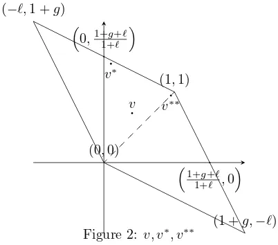
We have shown that two types of payoff vectors can be approximated by se-quential equilibria (Propositions 1 and 4) when the discount factor is sufficiently large and the observation cost is sufficiently small. It is straightforward to show that payoff vector(1+g+ℓ
1+ℓ ,0
)
Using the technique in Ellison (1994) again and alternating four strate-gies σ∗,σ˜, ˆσ, and the repetition of the stage game Nash equilibrium, we can approximate any payoff vector inF∗.
Theorem 1(Approximate folk theorem). Suppose that a public randomization is available, and Assumptions 1 and 2 are satisfied. Fix any interior point v= (v1, v2) of F∗. Fix any ε >0. There exist a discount factor δ∈( g
1+g,1
)
and observation costλ >0such that for anyδ∈[δ,1)andλ∈(0, λ), there exists a sequential equilibrium whose payoff vectorvF = (vF
1, v2F)satisfies|vFi −vi| ≤ε.
Proof of Theorem 1. See Appendix E.
Remark 3. Our approach can be applied under the monitoring structure of Flesch and Perea (2009) if a public randomization device is available. Our strategy is a variant of the grim trigger strategy. It means that players have no incentive to observe the opponent once after the punishment starts. In addition, in our strategy, playerichoosesCiand chooseDi if he is not in the cooperation
state. Therefore, the observation in the current period gives player i enough information to check whether the punishment starts or not. Therefore, each player does not have an incentive to acquire information about past actions.
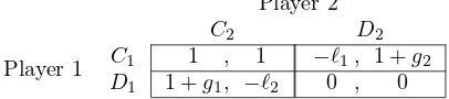
Remark 4. We have proven efficiency and the folk theorem in a repeated symmetric prisoner’s dilemma. In this section, we discuss what happens if the prisoner’s dilemma is asymmetric, as in Table 3.
Player 2
C2 D2
Player 1 C1 1 , 1 −ℓ1, 1 +g2
[image:18.612.207.410.412.457.2]D1 1 +g1, −ℓ2 0 , 0 Table 3: Asymmetric prisoner’s dilemma
In the proofs of the propositions and theorems below, we require that the discount factor δ is sufficiently close to 1+gg. This condition is required to approximate a Pareto-efficient payoff vector. If g1 ̸= g2, it is impossible to ensure that the discount factor δ is sufficiently close to both g1
1+g1 and
g2
1+g2.
Therefore, we have to confine our attention to the case ofg1=g2=g.
Let us consider Propositions 1 and 2. In the construction of the strategy, the randomization probability of playeriis defined based on the incentive con-straint of the opponent only. In other words, the randomization probability
is determined independently of the payoffs of player i. This means that the
randomization probability of player iis determined based on δ, g, ℓj and is
in-dependent of ℓi. Therefore, we can discuss the randomization probabilities of
player 1 and 2 independently. Hence, ifg1 =g2 and Assumptions 1 and 2 for
each ℓi (i = 1,2) hold, our efficiency result and folk theorem under a small
6
Concluding Remarks
Although only a few possible types of cooperation exist in a player, two-action prisoner’s dilemma, prisoner’s dilemma under costly monitoring is still a useful model to understand cooperation. Prisoner’s dilemma under costly monitoring has some properties. First, the number of actions is limited. This means that players cannot communicate using a variety of actions. Second, the number of players is limited. If there are three players A, B, C, it is easy
to check the observation deviation of the opponents. Player A can monitor
the observational decisions of players B andC by comparing their actions. If playersB andC choose inconsistent actions toward each other, player Afinds
that players B or C do not observe some of the players. Third, there is no
free-cost informative signal. To obtain information about the actions chosen by their opponents, players have to observe.
Originally, the prisoner’s dilemma under costly monitoring has these con-straints. Despite the above limitations, we have shown efficiency without any randomization device. Our paper is the first result to show that efficiency holds without any randomization device under an infinitely repeated prisoner’s dilemma with costly monitoring, although it is the simplest model among those with costly monitoring considered in the literature (e.g., Miyagawa et al. (2003) and Flesch and Perea (2009)).
We considered a public randomization device and obtained a folk theorem. It is worth mentioning that our folk theorem holds in some asymmetric prisoner’s dilemma. Our results can be applied to more general games.
A
Proof of Proposition 1
Proof. We prove Proposition 1.
Strategy
We define a grim trigger strategy σ∗, and then we define a consistent system of beliefsψ∗. Strategy σ∗ is represented by an automaton that has four types of states: initial stateω1
i, cooperation states (ωti)∞t=2, transition stateωEi , and
defection stateωD
i . For any period t≥2, there is a unique cooperation state.
Letωt
i be the cooperation state in periodt≥2.
At the initial state ω1
i, each player i chooses (Ci,1) with probability (1−
β1)(1−β2), chooses (Ci,0) with probability (1−β1)β2, and chooses (Di,0) with
probability β1. We call (ai, oi) an action–observation pair. The state moves
from the initial state to the cooperation stateω2
i if the action–observation pair
in period 1 is (Ci, Cj). The state moves to the transition state ωiE in period 2
when (Ci, ϕi) is realized in period 1. Otherwise, the state moves to a defection
state in period 2.
At the cooperation state ωt
i, each player i chooses (Ci,1) with
probability βt+1 depends on calendar time t. The state moves to the next
co-operation stateωti+1 if the action–observation pair in periodt is (Ci, Cj). The
state moves to the transition stateωE
i in period t+ 1 when (ati, oti) or (Ci, ϕi)
is realized in period t. Otherwise, the state moves to the defection state in periodt+ 1.
At the transition state ωE
i in period t, each player i chooses (Di,0) with
certainty. The state moves to the defection state ωD
i in period t+ 1 when
at
i = Di or oti = Dj is realized. If player i chooses (Ci,0), the state remains
the same. When player ichooses Ci and observes Cj in periodt, the state in
periodt+ 1 moves to the cooperation stateωt+1
i .
Players choose (Di,0) and the state remains the sameωDi at the defection
stateωD
i , irrespective of the action–observation pair.
The state-transition rule is summarized in Figure 1. Let strategyσ∗ be the strategy represented by the above automaton.
We define a system of beliefs consistent with strategy σ∗ by the same ap-proach as that in Section 4. Each behavioral strategy profile ˆσn induces the
system of beliefsψn, and the consistent system of beliefsψ∗ is defined as the limit of limn→∞ψn.
Selection of discount factor and observation cost
Fix anyε >0. We defineε,δ,δ, and λas follows
ε≡ ℓ
2
54(1 +g+ℓ)3 ε
1 +ε, δ≡ g
1 +g+ε, δ≡ g
1 +g+ 2ε <1,
λ≡ 1
16
g
1 +g
1 1 +g+ℓε
2.
We fix an arbitrary discount factor δ ∈ [δ, δ] and an arbitrary observation costλ∈(0, λ). We show that there exists a sequential equilibrium whose payoff vector (v∗
1, v∗2) satisfiesvi∗≥1−εfor eachi= 1,2.
Specification of strategy
Let us define ε′ ≡ δ− g
1+g. We set β1 =
1+g+ℓ g+ℓ ε
′. Given β1, we define β2 as the solution of the following indifference condition between (Ci,0) and (Di,0)
in period 1.
(1−β1)·1−β1·ℓ+δ(1−β1)(1−β2)(1 +g) =(1−β1)(1 +g). (3)
Next, we define (βt)∞t=3. We chooseβt+2so that playerjat stateωitis indifferent
To define βt(t ≥ 3), let Wt (t ≥ 1) be the sum of the stage game payoffs
from the cooperation stateωt
i. That is, payoffWt is given by
Wt=
[ ∞ ∑
s=t
δs−1u
i(as)
σ∗, ψ∗, ωt i
]
.
Please note that Wt (t ≥ 1) is determined uniquely. There are several
histories associated with the cooperation stateωt
i (e.g., the ones where playeri
cooperated and observed cooperation in the transition state in the previous period). At any of those histories, player i believes that player j is at the cooperation state ωt
j with probability 1−βt and at the transition state with
probabilityβt. Therefore, the continuation payoffWtis uniquely determined.
At the cooperation state ωt
i(t ≥2), playeri weakly prefers to play (Ci,0).
Therefore, payoffWtis given by
Wt= (1−βt)·1−βtℓ+δ(1−βt)(1−βt+1)(1 +g), ∀ t≥2. (4)
Therefore, payoff Wt is a function of (βt, βt+1). We denote payoff Wt by
Wt(βt, βt+1) when we should consider Wtas a function of (βt, βt+1).
Then,β3is given by
W1=(1−β1)·1−β1ℓ−λ+δ(1−β1)W2(β2, β3). (5)
Next, let us consider the indifference condition between (Ci,1) and (Ci,0)
at the cooperation stateωt
i(t≥2). Let us consider the belief for each playeri
at the cooperation stateωt
i in period t. Assume thatβt∈(0,1) for anyt∈N,
which is proved later. Then, we show by mathematical induction that, for any periodt≥2, playeri at the cooperation state ωt
i in period t believes that the
state of his opponent is a cooperation state with positive probability 1−βt. Let
us consider periodt = 2 first. The state moves to the cooperation stateω2
i in
period 2 only when playerihas observed the action–observation pair (a1
i, o1i) =
(Ci, Cj) in period 1. Therefore, playeribelieves that the state of his opponent
is the cooperation state with positive probability 1−β2 by Bayes’ rule. Thus, the statement is true in period 2. Next, suppose that the statement is true until periodtand consider playeri at the cooperation state ωit+1. This means that player i has observed action–observation pair (at
i, oti) = (Ci, Cj) in period t.
Thus, playeribelieves with certainty that playerjwas in the cooperation state in periodt. Therefore, he believes that playerj is the in the cooperation state with positive probability 1−βt+1 by Bayes’ rule. Hence, the statement is true.
Taking the belief at the cooperation state ωt
i(t ≥ 2) into account, βt+2 is
defined as the solution of the equation below.
Specifically,β2is defined by (3), andβt+2(t∈N) is defined by (6) as follows.
β2=(1−β1){δ(1 +g)−g} −β1ℓ
δ(1−β1)(1 +g)
= g+g
2−ℓ2−(1 +g+ℓ)(1 +g)ε′ (g+ℓ){g+ (1 +g)ε′}(1−1+g+ℓ
g+ℓ ε′
)ε
′
=1 +g−
ℓ
gℓ−(1 +g+ℓ)
1+g g ε
′
1 + ℓ g
1
g+ℓε′−
(1+g)(1+g+ℓ)
g(g+ℓ) (ε′)2
1
g+ℓε
′
βt+2=
(1−βt+1){δ(1 +g)−g} −βt+1ℓ−δ(1−λβt)
δ(1−βt+1)(1 +g)
, ∀t∈N.
Now, to focus on a game theoretic argument, we assume the following Lemma 2, which is proved in Appendix B.
Lemma 2. Suppose that Assumptions 1 and 2 are satisfied. Fix any discount factorδ∈[δ, δ]and observation cost λ∈(0, λ). Then, it holds that
1 2
1 +g−ℓ g+ℓ ε
′< β2< β4< β6· · ·< β5< β3< β1= 1 +g+ℓ
g+ℓ ε
′.
Thanks to Lemma 2, we obtain a lower bound and an upper bound of βt for
anyt∈N.
Now, let us show that the grim trigger strategyσ∗is a sequential equilibrium.
Sequential rationality at the initial state
At the initial state, the indifference condition between (Ci,0) and (Di,0) is
ensured by the construction ofβ2. The indifference condition between (Ci,1)
and (Ci,0) is ensured by the construction ofβ3. Furthermore, if playerichooses
action Di, then his opponent chooses action Dj with certainty from the next
period on, irrespective of his observation result. Thus, playerihas no incentive to choose (Di,1). Therefore, it is optimal for player i to follow strategyσ∗ at
the initial state.
Sequential rationality in the cooperation state
Next, consider a history associated with the cooperation stateωt
i in periodt(≥
2). Then, strategy σ∗ prescribes to randomize (C
i,1) and (Ci,0). As we
explained earlier, at any history associated with a cooperation state in pe-riod t (≥ 2), player i believes that player j is at the cooperation state ωt j
with probability 1−βt and at the transition state with probability βt. The
definition ofβt+2 ensures that (Ci,1) and (Ci,0) are indifferent for playeri in
is bounded above by (1−βt)(1 +g). Equation (6) implies that, for any t∈N,
it holds that
Wt+1= (1−βt+1)(1 +g) + λ δ(1−βt)
. (7)
The above equality ensures that, for any period t ≥ 1, (1−βt+1)(1 +g) is
strictly smaller thanWt+1, which is the payoff when playerichooses (Ci,1) in
periodt+ 1. Thus, both (Di,0) and (Di,1) are suboptimal in any periodt≥2.
Therefore, it is optimal for player i to follow strategy σ∗ in the cooperation state.
Sequential rationality at the defection state
Consider any history associated with the defection state. Then, σ∗ prescribes (Di,0). Since we consider the belief construction similar to the one in Miyagawa
et al. (2008), player i believes that player j never deviates from prescribed observational decision as the same as Miyagawa et al. (2008). Therefore, playeri
is certain that the state of his opponent is either the transition or defection state, and playeri’s action in that period does not affect the continuation play of his opponent. Furthermore, playeribelieves that playerj chooses actionDj with
certainty and has no incentive to observe his opponent. Therefore, it is optimal for playerito follow strategyσ∗ in the defection state.
Sequential rationality in the transition state
We consider any history in periodt (≥2) associated with the transition state. Strategyσ∗ prescribes (D
i,0) in the transition state.
Let us consider a continuation payoff when player i chooses action Ci in
periodt. Letpbe the belief of playeriin the transition state in periodt that his opponent is in the cooperation state. If playeriobserves his opponent, then (at
i, oti) = (Ci, Cj) is realized with probability p and the state moves to the
cooperation state (ωit+1). The continuation payoff in the cooperation state in periodt+ 1 is bounded above byWt+1. This is becauseWt+1 is a continuation
payoff when playerichooses action Ci from ωit+1, andWt+1 is strictly greater
than payoff (1−βt+1)(1 +g), which is the upper bound of the payoff when
player i chooses action Di at ωit+1. Therefore, the upper bound of the
non-averaged payoff when playerichooses actionCi in periodtis given by
p−(1−p)ℓ+δpWt+1.
The non-averaged payoff when playerichoosesDiis bounded above byp(1+g).
Therefore, actionDi is profitable if the following value is negative.
We can rewrite the above value as follows.
p−(1−p)ℓ+δpWt+1−p(1 +g)
=(1−βt)−βtℓ−λ+δ(1−βt)Wt+1−(1−βt)(1 +g)
+λ+{p−(1−βt)} {1 +ℓ+δWt+1−(1 +g)}
=Wt−(1−βt)(1 +g) +λ+{p−(1−βt)} {δWt+1−(g−ℓ)}
= λ
δ(1−βt−1)
+λ+{p−(1−βt)} {δWt+1−(g−ℓ)}. (8)
The second equality follows from equation (6) in periodt. The last equality is ensured by (7) in periodt−1.
Using equation (7), we obtain the lower bound ofδWt+1−(g−ℓ) as follows. δWt+1−(g−ℓ)≥δ(1−βt+1)(1 +g)−(g−ℓ)
≥ {g+ (1 +g)ε′}
(
1−1 +g+ℓ
g+ℓ ε
′
)
−(g−ℓ)
≥ℓ
2. (9)
The second inequality follows fromβt≤1+g+g+ℓℓε′by Lemma 2. The last
inequal-ity is ensured byε′ ≤2ε. The maximum value ofpis (1−β
t−1)(1−βt). Taking
(9) into account, we show that (8) is negative as follows.
λ δ(1−βt−1)
+λ− {(1−βt)−p} {δWt+1−(g−ℓ)}
≤ λ
δ(1−βt−1)
+λ−(1−βt)βt−1 ℓ
2
≤1 +g
g
1
1−1+g+g+ℓℓε′λ+λ−
(
1−1 +g+ℓ
g+ℓ ε
′
)1
2
1 +g−ℓ g+ℓ ε
′ℓ 2
<0.
The second inequality is ensured by δ ∈ [δ, δ] by Lemma 2 and βt, βt−1 ∈
[
1 2
1+g−ℓ g+ℓ ε
′,1+g+ℓ g+ℓ ε
′]. Therefore, player iprefers D
i to Ci. Hence, it has been
proven that it is optimal for playerito follow strategy σ∗. The strategy σ∗ is a sequential equilibrium.
The payoff
Finally, we show that the sequential equilibrium payoff v∗
i is strictly greater
than 1−ε. Player ichooses (Di,0) in period 1 at the initial state. Therefore,
the equilibrium payoffv∗
i is given by
v∗i = (1−δ)(1−β1)(1 +g) ={1−(1 +g)ε′}
(
1−1 +g+ℓ
g+ℓ ε
′)>1−ε.
B
Proof of Lemma 2
Proof of Lemma 2. To prove Lemma 2, we will use the following Lemma 3 holds.
Lemma 3. Suppose that Assumptions 1 and 2 are satisfied. Fix any discount factor δ∈ [δ, δ] and observation cost λ ∈(0, λ). Then, β1−β2 ≥ g+ℓℓε′ holds and, for anyt∈N, it holds that
0< ℓ
2g <−
βt+2−βt+1 βt+1−βt
<1.
Assume that Lemma 3 holds. Usingβt,βt+1, and−ββt+2t+1−−βtβ+1t , we can express βt+2as follows.
βt+2=βt+ (βt+1−βt) + (βt+2−βt+1)
=βt+ (βt+1−βt)
{
1−
(
−βt+2−βt+1
βt+1−βt
)}
=
(
−βt+2−βt+1
βt+1−βt
)
βt+
{
1−
(
−βt+2−βt+1
βt+1−βt
)}
βt+1.
Therefore, ifβt, βt+1∈[0,1], and 2ℓg <−ββt+2t −βt+1
+1−βt <1 hold, we obtainβt+2∈ (min{βt, βt+1},max{βt, βt+1}) becauseβt+2 is a convex combination ofβtand
βt+1.
Let us compare β1, β2, and β3. By Lemma 3, β1 −β2 is greater than
ℓ g+ℓε
′. Furthermore, we have β2 < β3 < β1 because −(−βt+2−βt+1
βt+1−βt
)
∈ (0,1)
by Lemma 3 and, then,β3 is a convex combination of β1 and β2. Next, let us
compareβ2,β3, and β4. As we find,β2 is smaller thanβ3. Therefore, we have
β2 < β4 < β3 because β4 is a convex combination ofβ2 and β3. Similarly, for anys∈N, it holds that (β2s<)β2s+1< β2s−1, andβ2s< β2s+2(< β2s+1).
Next, we prove Lemma 3.
Proof of Lemma 3. First, let us derive−β3−β2
β2−β1. By (3), we have
0 =−(1−β1)g−β1ℓ+δ(1 +g)(1−β1)(1−β2). (10)
Furthermore, by (4) and (5), we have
λ
δ(1−β1) =−(1−β2)g−β2ℓ+δ(1 +g)(1−β2)(1−β3) (11)
By (10) and (11), we obtain
(β2−β1)(g−ℓ)−δ(1 +g)(1−β2){(β3−β2) + (β2−β1)}= λ
Let us consider the lower bound ofβ2. As ε′ ∈[ε,2ε] and 0< ℓ
g <1 hold, we
have
β2=1 +g−
ℓ
gℓ−(1 +g+ℓ)
1+g g ε
′
1 + ℓ g
1
g+ℓε′−
(1+g)(1+g+ℓ)
g(g+ℓ) (ε′)2
1
g+ℓε
′
> 3
4(1 +g−ℓ) 3 2
1
g+ℓε >
1 2
1 +g+ℓ g+ℓ ε
′.
Next, let us consider the upper bound ofβ2.
β2=1 +g−
ℓ
gℓ−(1 +g+ℓ)
1+g g ε
′
1 +gℓg+1ℓε′−(1+g)(1+g+ℓ)
g(g+ℓ) (ε′)2
1
g+ℓε
′
< 1 +g−
ℓ g
1−(1+gg()(1+g+ℓg)+ℓ)(ε′)2
1
g+ℓε
′
< 1 +g−
ℓ g
1−(1+gg)(1+(g+ℓ)g+ℓ)ε′ 1
g+ℓε
′ <1 +g
g+ℓε
′.
The last inequality is ensured byε′<2ε. Thus, we obtain 1
2
1 +g−ℓ g+ℓ ε
′ < β2<1 +g
g+ℓε
′.
Asβ2<1+g+gℓε′ < β1=1+g+ℓ g+ℓ ε
′, we can divide both sides of (12) byβ2−β1and obtain−β3−β2
β2−β1.
−β3−β2
β2−β1 =
ℓ+δ(1 +g)(1−β2)−g+ λ δ(1−β1)(β2−β1)
δ(1 +g)(1−β2) .
As Assumption 2,β1, β2<1, andβ2−β1<0 hold, we find an upper bound of
−β3−β2
β2−β1.
−β3−β2
β2−β1 ≤
δ(1 +g)(1−β2) + λ δ(1−β1)(β2−β1)
δ(1 +g)(1−β2) <1. Taking β1 = 1+g+g+ℓℓε′, β2 < 1+g
g+ℓε′, and −(β2−β1) > ℓ
g+ℓε′ into account, we
have a lower bound of−β3−β2
β2−β1 as follows.
−β3−β2
β2−β1 >
ℓ+g(1−1+g+gℓε′)−g− ℓ
( g
1+g+ε′)(1− 1+g+ℓ
g+ℓ ε′)
λ ε′ (
g
1+g +ε′
)
(1 +g)
>
ℓ−1+g+gℓgε′− ℓ
( g
1+g+ε′)(1− 1+g+ℓ
g+ℓ ε′)
λ ε′
g+ (1 +g)ε′
> 3 4ℓ 3 2g > ℓ
The first inequality follows fromδ = 1+gg +ε′ > g
1+g. The third inequality is
ensured byε′ <2εand λ < λ. Therefore, we have obtained 2ℓg <−β3−β2
β2−β1 <1
andβ3∈(β2, β2). That is,β3−β2>0. Next, let us derive−βt+3−βt+2
βt+2−βt+1inductively. Suppose that
ℓ
2g <−
βs+2−βs+1
βs+1−βs < 1 and βs+2 ∈ (min{βs, βs+1},max{βs, βs+1}) hold for period s = 1,2, . . . , t.
We have shown that this supposition holds for t = 1. We show that ℓ
2g <
−βt+3−βt+2
βt+2−βt+1 <1 andβt+3∈(min{βt+1, βt+2},max{βt+1, βt+2}) hold.
By (4), (5), and (6), for anyt∈N, we have
{ λ
δ(1−βt) =−(1−βt+1)g−βt+1ℓ+δ(1−βt+1)(1−βt+2)(1 +g)
λ
δ(1−βt+1)=−(1−βt+2)g−βt+2ℓ+δ(1−βt+2)(1−βt+3)(1 +g),
or,
− βt+1−βt
δ(1−βt)(1−βt+1)λ
=−(βt+2−βt+1)(g−ℓ) +δ(1−βt+2){(βt+3−βt+2) + (βt+2−βt+1)}(1 +g).
The suppositions ensureβt+2−βt+1̸= 0. Divide both sides of the above equation
byβt+2−βt+1. Then, we obtain
−βt+3−βt+2
βt+2−βt+1
=
ℓ+δ(1 +g)(1−βt+2)−g+ 1
δ(1−βt)(1−βt+1)βt+2
−βt+1 βt+1−βt
λ
δ(1 +g)(1−βt+2)
. (13)
As Assumption 2 and βt+2−βt+1
βt+1−βt <0 hold,−
βt+3−βt+2
βt+2−βt+1 is bounded above by
−βt+3−βt+2
βt+2−βt+1
≤
δ(1 +g)(1−βt+2) + 1
δ(1−βt)(1−βt+1)βt+2
−βt+1 βt+1−βt
λ
δ(1 +g)(1−βt+2)
<1.
Taking 0< βt+1, βt+2 <1+g+g+ℓℓε
′=β1, and ℓ
2g <−
βt+2−βt+1
βt+1−βt <1 into account, we find the following lower bound of−βt+3−βt+2
βt+2−βt+1.
−βt+3−βt+2
βt+2−βt+1
=
ℓ+δ(1−βt+2)(1 +g)−g+ 1
δ(1−βt)(1−βt+1)βt+2
−βt+1 βt+1−βt
λ
δ(1 +g)(1−βt+2)
>
ℓ+g(1−1+g+g+ℓℓε′)−g− 1
( g
1+g+ε′)(1− 1+g+ℓ
g+ℓ ε′) 2 2g
ℓ
λ
(
g
1+g+ε′
)
(1 +g)
>
ℓ−1+g+g+ℓℓgε′− 1
g 1+g·
1 4·2ε
′
g+ (1 +g)ε′ >
3 4ℓ 3 2g
> ℓ
2g.
Therefore, we obtained ℓ
2g <−
βt+3−βt+2
C
Proof of Proposition 3
Proof of Proposition 3 . By (13), we have
−βt+3−βt+2
βt+2−βt+1
=1− g−ℓ
δ(1−βt+2)(1 +g)
− 1
δ2(1−β
t)(1−βt+1)(1−βt+1)ββt+2t+1−−βtβ+1t λ.
Therefore, ifg−ℓ < 0 and λis small, then −βt+3−βt+2
βt+2−βt+1 > 1, and|βt| goes to
infinity astgoes to infinity. That is, we have obtained a necessary condition for the efficiency result.
D
Proof of Proposition 4
Proof. Fix anyε >0. We define ε,δ,δ, andλas follows:
ε≡ ℓ
2
54(1 +g+ℓ)2 ε
1 +ε, δ≡ g
1 +g+ε, δ≡ g
1 +g+ 2ε,
λ≡ 1
16
g
1 +g
1 1 +g+ℓε
2.
Fix any δ ∈ [
δ, δ]
and λ ∈ (0, λ). We show a sequential equilibrium whose
payoff vector (v∗1, v∗2) satisfiesv1∗= 0 andv2∗≥ 1+g+ℓ
1+ℓ −ε.
Strategy
We define a grim trigger strategy ˜σ. Strategy ˜σis represented by an automaton that has four types of states: initial ˜ω1
i, cooperation (˜ωit)∞t=2, transition ωiE,
and defection ωD
i . Players use the public randomization only at the initial
state.
At the initial state ˜ω1
1, player 1 chooses C1 with probability 1−β1,1 and D1 with probability β1,1. Player 1 does not observe player 2 irrespective of
his action. The transition state depends on a realized sunspot. If the realized sunspot is greater than ˆx, the state remains the same. If the realized sunspot is not greater than ˆxand player 1 choosesC1, then the state in the next period moves to the cooperation state ˜ω2
1. If the realized sunspot is not greater than ˆx
and player 1 choosesD1, then the s