5692
Word2Sense : Sparse Interpretable Word Embeddings
Abhishek Panigrahi Microsoft Research India
Harsha Vardhan Simhadri Microsoft Research India
Chiranjib Bhattacharyya Microsoft Research India, and
Indian Institute of Science [email protected]
Abstract
We present an unsupervised method to gener-ate Word2Sense word embeddings that are interpretable — each dimension of the em-bedding space corresponds to a fine-grained
sense, and the non-negative value of the em-bedding along thej-th dimension represents the relevance of the j-th sense to the word. The underlying LDA-based generative model can be extended to refine the representation of a polysemous word in a short context, allowing us to use the embeddings in con-textual tasks. On computational NLP tasks, Word2Sense embeddings compare well with other word embeddings generated by unsuper-vised methods. Across tasks such as word sim-ilarity, entailment, sense induction, and con-textual interpretation, Word2Sense is compet-itive with the state-of-the-art method for that task. Word2Sense embeddings are at least as sparse and fast to compute as prior art.
1 Introduction
Several unsupervised methods such as SkipGram (Mikolov et al., 2013) and Glove (Pennington et al., 2014) have demon-strated that co-occurrence data from large corpora can be used to compute low-dimensional repre-sentations of words (a.k.a. embeddings) that are useful in computational NLP tasks. While not as accurate as semi-supervised methods such as BERT (Devlin et al.,2018) andELM O (Peters et al., 2018) that are trained on various down-stream tasks, they do not require massive amounts of compute unaccessible to all but few.
Nearly all such methods produce dense repre-sentations for words whose coordinates in them-selves have no meaningful interpretation. The nu-merical values of a word’s embedding are mean-ingful only in relation to representations of other words. A unitary rotation can be applied to many
of these embeddings retaining their utility for computational tasks, and yet completely chang-ing the values of individual coordinates. Can we design an interpretable embedding whose coordi-nates have a clear meaning to humans?
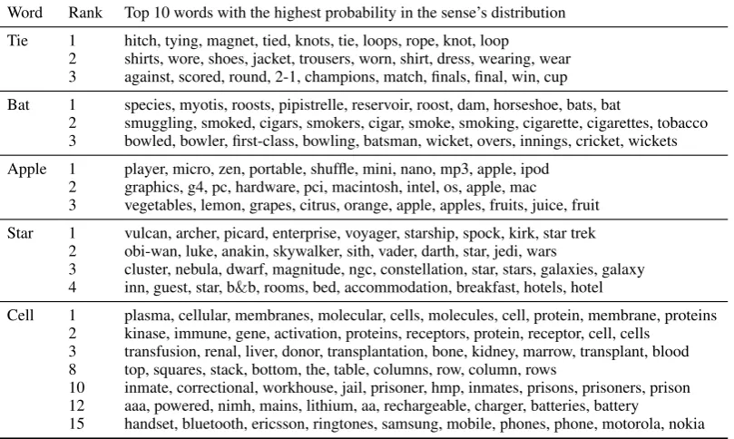
Ideally such an embedding would capture the multiplesensesof a word, while being effective at computational tasks that use inter-word spacing of embeddings. Loosely, a sense is a set of semanti-cally similar words that collectively evoke a bigger picture than individual words in the reader’s mind. In this work, we mathematically define a sense to be a probability distribution over the vocabulary, just as topics in topic models. A human can re-late to a sense through the words with maximum probability in the sense’s probability distribution.
Table 1presents the top 10 words for a few senses. We describe precisely such an embedding of words in a space where each dimension corre-sponds to a sense. Words are represented as prob-ability distributions over senses so that the magni-tude of each coordinate represents the relative im-portance of the corresponding sense to the word. Such embeddings would naturally capture the pol-ysemous nature of words. For instance, the em-bedding for a word such ascellwith many senses – e.g. “biological entity”, “mobile phones”, “ex-cel sheet”, “blocks”, “prison” and “battery” (see
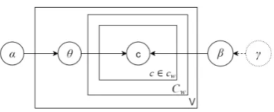
Table 1) – will have support over all such senses. To recover senses from a corpus and to repre-sent word embeddings as (sparse) probability dis-tributions over senses, we propose a generative model (Figure 1) for the co-occurrence matrix: (1) associate with each word w a sense distribution θwwith Dirichlet prior; (2) form a context around
a target word w by sampling senses z according toθw, and sample words from the distribution of
cor-Word Rank Top 10 words with the highest probability in the sense’s distribution
Tie 1 hitch, tying, magnet, tied, knots, tie, loops, rope, knot, loop
2 shirts, wore, shoes, jacket, trousers, worn, shirt, dress, wearing, wear 3 against, scored, round, 2-1, champions, match, finals, final, win, cup
Bat 1 species, myotis, roosts, pipistrelle, reservoir, roost, dam, horseshoe, bats, bat
2 smuggling, smoked, cigars, smokers, cigar, smoke, smoking, cigarette, cigarettes, tobacco 3 bowled, bowler, first-class, bowling, batsman, wicket, overs, innings, cricket, wickets
Apple 1 player, micro, zen, portable, shuffle, mini, nano, mp3, apple, ipod 2 graphics, g4, pc, hardware, pci, macintosh, intel, os, apple, mac
3 vegetables, lemon, grapes, citrus, orange, apple, apples, fruits, juice, fruit
Star 1 vulcan, archer, picard, enterprise, voyager, starship, spock, kirk, star trek 2 obi-wan, luke, anakin, skywalker, sith, vader, darth, star, jedi, wars
3 cluster, nebula, dwarf, magnitude, ngc, constellation, star, stars, galaxies, galaxy 4 inn, guest, star, b&b, rooms, bed, accommodation, breakfast, hotels, hotel
Cell 1 plasma, cellular, membranes, molecular, cells, molecules, cell, protein, membrane, proteins 2 kinase, immune, gene, activation, proteins, receptors, protein, receptor, cell, cells
3 transfusion, renal, liver, donor, transplantation, bone, kidney, marrow, transplant, blood 8 top, squares, stack, bottom, the, table, columns, row, column, rows
10 inmate, correctional, workhouse, jail, prisoner, hmp, inmates, prisons, prisoners, prison 12 aaa, powered, nimh, mains, lithium, aa, rechargeable, charger, batteries, battery
[image:2.595.99.504.64.306.2]15 handset, bluetooth, ericsson, ringtones, samsung, mobile, phones, phone, motorola, nokia
Table 1: Top senses of polysemous words as identified Word2Sense embeddings. Each row lists the rank of the sense in terms of its weight in the word’s embedding, and the top 10 words in the senses’ probability distribution.
pora and construct the embeddings.
W ord2Sense embeddings are extremely sparse despite residing in a higher dimensional space (few thousand), and the number of non-zeros in the embeddings is no more than100. In comparison, W ord2vec performs best on most tasks when computed in 500 dimensions.
These sparse single prototype embeddings ef-fectively capture the senses a word can take in the corpus, and can outperform probabilistic em-beddings (Athiwaratkun and Wilson, 2017) at tasks such as word entailment, and compete with W ord2vec embeddings and multi-prototype em-beddings (Neelakantan et al., 2015) in similarity and relatedness tasks.
Unlike prior work such as W ord2vec and GloVe, our generative model has a natural exten-sion for disambiguating the senses of a polyse-mous word in a short context. This allows the re-finement of the embedding of a polysemous word to aW ordCtx2Sense embedding that better re-flects the senses of the word relevant in the text. This is useful for tasks such as Stanford con-textual word similarity (Huang et al., 2012) and word sense induction (Manandhar et al.,2010).
Our methodology does not suffer from com-putational constraints unlike W ord2GM ( Athi-waratkun and Wilson, 2017) and M SSG ( Nee-lakantan et al., 2015) which are constrained to
learning 2-3 senses for a word. The key idea that gives us this advantage is that rather than con-structing a per-word representation of senses, we construct a global pool of senses from which the senses a word takes in the corpus are inferred. Our methodology takes just 5 hours on one mul-ticore processor to recover senses and embeddings from a concatenation of UKWAC (2.5B tokens) and Wackypedia (1B tokens) co-occurrence ma-trices (Baroni et al., 2009) with a vocabulary of 255434words that occur at least100times.
Our major contributionsinclude:
• A single prototype word embedding that en-codes information about the senses a word takes in the training corpus in a human interpretable way. This embedding outperforms W ord2vec in rare word similarity task and word relatedness task and is within 2% in other similarity and re-latedness tasks; and outperformsW ord2GMon the entailment task of (Baroni et al.,2012). • A generative model that allows for
2 Related Work
Several unsupervised methods generate dense single prototype word embeddings. These include W ord2vec (Mikolov et al., 2013), which learns embeddings that maximize the co-sine similarity of embeddings of co-occurring words, and Glove (Pennington et al., 2014) and Swivel (Shazeer et al., 2016) that learn embed-dings by factorizing the word co-occurrence ma-trix. (Dhillon et al., 2015; Stratos et al., 2015) use canonical correlation analysis (CCA) to learn word embeddings that maximize correlation with context. (Levy and Goldberg, 2014; Levy et al.,
2015) showed that SVD based methods can com-pete with neural embeddings. (Lebret and Col-lobert, 2013) use Hellinger PCA, and claim that Hellinger distance is a better metric than Eu-clidean distance in discrete probability space.
Multiple works have considered converting the existing embeddings to interpretable ones. Mur-phy et al. (2012) use non-negative matrix factor-ization of the word-word co-occurrence matrix to derive interpretable word embeddings. (Sun et al.,
2016;Han et al.,2012) change the loss function in Glove to incorporate sparsity and non negativity respectively to capture interpretability. (Faruqui et al., 2015) propose Sparse Overcomplete Word Vectors (SP OW V), by solving an optimization problem in dictionary learning setting to produce sparse non-negative high dimensional projection of word embeddings. (Subramanian et al.,2018) use ak-sparse denoising autoencoder to produce sparse non-negative high dimensional projection of word embeddings, which they called SParse In-terpretable Neural Embeddings (SP IN E). How-ever, all these methods lack a natural extension for disambiguating the sense of a word in a context.
In a different line of work, Vilnis and McCal-lum(2015) proposed representing words as Gaus-sian distributions to embed uncertainty in dimen-sions of the embedding to better capture concepts like entailment. However, Athiwaratkun and Wil-son (2017) argued that such a single prototype model can’t capture multiple distinct meanings and proposedW ord2GMto learn multiple Gaus-sian embeddings per word. The prototypes were generalized to ellipical distributions in (Muzellec and Cuturi, 2018). A major limitation with such an approach is the restriction on the number of prototypes per word that can be learned, which is limited to 2 or 3 due to computational constraints.
Many words such as ‘Cell’ can have more than 5 senses. Another open issue is that of disambiguat-ing senses of a polysemous word in a context – there is no obvious way to embed phrases and sen-tences with such embeddings.
Multiple works have proposed multi-prototype embeddings to capture the senses of a polysemous word. For example, Neelakantan et al.(2015) ex-tends the skipgram model to learn multiple em-beddings of a word, where the number of senses of a word is either fixed or is learned through a non-parametric approach. Huang et al. (2012) learns multi-prototype embeddings by clustering the context window features of a word. However, these methods can’t capture concepts like entail-ment. Tian et al.(2014) learns a probabilistic ver-sion of skipgram for learning multi-sense embed-dings and hence, can capture entailment. How-ever, all these models suffer from computational constraints and either restrict the number of pro-totypes learned for each word to 2-3 or restrict the words for which multiple prototypes are learned to the topkfrequent words in the vocabulary.
Prior attempts at representing polysemy in-clude (Pantel and Lin,2002), who generate global senses by figuring out the best representative words for each sense from co-occurrence graph, and (Reisinger and Mooney, 2010), who gener-ate senses for each word by clustering the con-text vectors of the occurrences of the word. Fur-ther attempts include Arora et al.(2018), who ex-press single prototype dense embeddings, such as W ord2vec andGlove, as linear combinations of sense vectors. However, their underlying linearity assumption breaks down in real data, as shown by
Mu et al. (2017). Further, the linear coefficients can be negative and have values far greater than1 in magnitude, making them difficult to interpret.
Neelakantan et al.(2015) and Huang et al.(2012) represent a context by the average of the embed-dings of the words to disambiguate the sense of a target word present in the context. On the other hand, Mu et al.(2017) suggest representing sen-tences as a hyperspace, rather than a single vector, and represent words by the intersection of the hy-perspaces representing the sentences it occurs in.
A number of works use na¨ıve Bayesian method (Charniak et al., 2013) and topic models (Brody and Lapata, 2009; Yao and Van Durme, 2011;
in-Figure 1: Generative model for co-occurrence matrix. Dirichlet priorγis used in WarpLDA.
stance of a word within a context as a pseudo-document, and achieve state of the art results in WSI task (Manandhar et al.,2010). Since this ap-proach requires training a single topic model per target word, it does not scale to all the words in the vocabulary.
In a different line of work, (Tang et al., 2014;
Guo and Diab,2011;Wang et al.,2015;Tang et al.,
2015;Xun et al.,2017) transform topic models to learn local context level information through sense latent variable, in addition to the document level information through topic latent variable, for pro-ducing more fine grained topics from the corpus.
3 Notation
LetV ={w1, w2, ..w|V|}denote the set of unique
tokens in corpus (vocabulary). Let C denote the word-word co-occurrence matrix constructed from the corpus, i.e., Cij is the number of times
wj has occurred in the context ofwi. We define a
context around a tokenwas the set ofnwords to the left andnwords to the right ofw. We denote the size of context window byn. Typicallyn= 5. Our algorithm uses LDA to infer asense model β – essentially a set ofkprobability distributions overV – from the corpus. It then uses the sense model to encode a word w as a k0-dimensional µ-sparse vector θw. Here, we use α and γ,
re-spectively, to denote the Dirichlet priors ofθw, the
sense distribution of a word w, and βz, context
word distribution in a sensez. J S is ak×k ma-trix that measures the similarity between senses. We denote thezthrow of a matrixM byMz.
4 Recovering senses
To recover senses, we suppose the following gen-erative model for generating words in a context of sizen(seeFigure 1).
1. For each wordw∈V, generate a distribution over sensesθwfrom the Dirichlet distribution
with priorα.
2. For each context cw around target word w,
and for each of the2ntokens ∈ cw, do
(a) Sample sensez∼M ultinomial(θw).
(b) Sample tokenc∼M ultinomial(βzn).
Such a generative model will generate a co-occurrence matrix C that can also be generated by another model. C is a matrix whose columns Cw are interpreted as a document formed from
the count of all the tokens that have occurred in a context centered at w. Given a Dirichlet prior of parameterαon sense distribution ofCwandβ,
the distribution over context words for each sense, documentCw (and thus the co-occurrence matrix
C) is generated as follows:
1. Generateθw ∼Dirichlet(α).
2. RepeatN times to generateCw:
(a) Sample sensez∼M ultinomial(θw).
(b) Sample tokenc∼M ultinomial(βz).
Based on this generative model, given the co-occurrence matrix C, we infer the matrixβ and the maximum aposteriori estimate θw for each
word using a fast variational inference tool such as WarpLDA (Chen et al.,2016).
5 W ord2Sense embeddings
W ord2Sense embeddings are probability distri-butions over senses. We discuss how to use the senses recovered by inference on the generative model insection 4to construct word embeddings. We demonstrate that the embeddings so computed are competitive with various multi-modal embed-dings in semantic similarity and entailment tasks.
5.1 ComputingW ord2Sense embeddings
Denote the probability of occurrence of a word in the corpus by p(w). We approximate the proba-bility of the word p(w)by its empirical estimate kCwk1/P
w0∈V kCw0k1. We define the global
probabilitypZ(z) of a sensez as the probability
that a randomly picked token in the corpus has that sense in it’s context window. We approximate the global distribution of generated senses using the following formulation.
pZ(z) =
X
w∈V
[image:4.595.84.279.66.146.2]Then, for each wordw ∈ V, we computepc(w),
its sense distribution (when acting as a context word) as follows:
pc(z|w) =
p(w|z)pZ(z)
p(w) =
βw,zpZ(z)
p(w) .
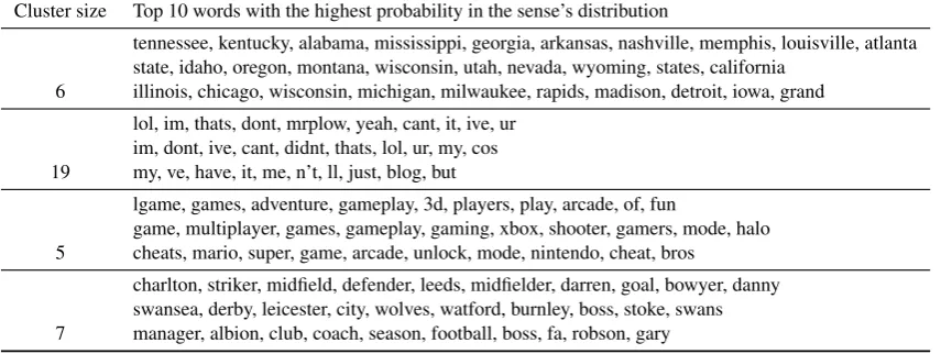
Eliminating redundant senses. LDA returns a number of topics that are very similar to each other. Examples of such topics are given in Ta-ble 11 in appendix. These topics need to be merged, since inferring two similar words against such senses can cause them to be (predominantly) assigned to two different topic ids, causing them to look more dissimilar than they actually are. In or-der to eliminate redundant senses, we use the sim-ilarity of topics according to the Jensen Shannon (JS) divergence. We construct the topic similarity matrixJ S∈Rk×k, whose[i, j]−thentryJ S[i, j]
is the JS divergence between sensesβiandβj.
Re-call that JS divergence J Sdiv(p, q) between two multinomial distributionsp, q∈Rkis given by
k
X
i=1
−pilog 2pi pi+qi
−qilog
2qi
pi+qi
. (1)
We run agglomerative clustering on theJ S ma-trix to merge similar topics. We use the following distance metric to merge two clustersDiandDj:
d(Di, Dj) =
1 |Di||Dj|
X
a∈Di, b∈Dj
J S[a, b]0.5
LetDi=1..k0 denote the final set ofk0 clusters
ob-tained after clustering. We approximate the occur-rence probability of the merged cluster of senses Di by pD(Di) = Pa∈DipZ(a).Table 11in
ap-pendix shows some clusters formed after cluster-ing. Using the merged senses, we compute the em-beddingvwof wordw— a distribution over senses
indexed byz∈ {1..k}— as follows:
ˆ
vw[z] =pc(z|w) +θw[z]
vw0 =T runcateµ(P roject(ˆvw)pD(.))
vw =vw0 /||v0w||1. (2)
P roject is the function that maps v ∈ Rk to
v0 ∈Rk0
by merging the coordinates correspond-ing to the merged senses: v0[i] = P
a∈Div[a].
T runcateµsparsifies the input by truncating it to
theµhighest non-zeros in the vector.
5.2 Evaluation
We compareW ord2Sense embeddings with the state-of-the-art on word similarity and entailment tasks as well as on benchmark downstream tasks. 5.2.1 Hyperparameters
We trainW ord2vecSkip-Gram embeddings with 10 passes over the data, using separate embed-dings for the input and output contexts, 5 nega-tive samples per posinega-tive example, window size n = 2 and the same sub-sampling and dynamic window procedure as in (Mikolov et al., 2013). ForW ord2GM, we make 5 passes over the data (due to very long training time of the published code 1), using 2 modes per word, 1 negative sample per positive example, spherical covari-ance model, window size n = 10 and the same sub-sampling and dynamic window procedure as in (Athiwaratkun and Wilson,2017). Since there is no recommended dimension in these papers, we report the numbers for the best performing embedding size. We report the performance of W ord2vecandW ord2GMat dimension 500 and 400 respectively2. We report the performance ofSP OW V and SP IN E in benchmark down-stream tasks, that useW ord2vecas base embed-dings, using the recommended settings as given in (Faruqui et al.,2015) and (Subramanian et al.,
2018) respectively3. For Multi-Sense Skip-Gram model (MSSG) (Neelakantan et al.,2015), we use pre-trained word and sense representations4.
We foundk= 3000, α= 0.1andγ = 0.001to be good hyperparamters for WarpLDA to recover fine-grained senses from the corpus. A choice of k0 ≈ 34k that merges k/4 senses improved re-sults. We use a context window size n = 5 and truncation parameter µ = 75. We thinkµ = 75 works best because we found the average sparsity ofpc(.|w)to be around 100. Since we decrease the
number of senses by1/4th after post-processing, the average sparsity reduces to close to 75. If a word is not present in the vocabulary, we take an embedding on the unit simplex, that contains equal values in all the dimensions.
5.2.2 Word Similarity
We evaluate our embeddings at scoring the simi-larity or relatedness of pairs of words on several
1
https://github.com/benathi/word2gm
2
We tried 100, 200, 300, 400, 500 dimensions for W ord2vec, and 50, 100, 200, 400 dims forW ord2GM
3
The two models don’t perform better thanW ord2vecin similarity tasks and don’t show performance in entailment.
Dataset Word Word W ord2GM MSSG 300-dim
2Sense 2Vec 30K 6K
WS353-S 0.747 0.769 0.756(0.767) 0.753 0.761 WS353-R 0.708 0.703 0.609(0.717) 0.598 0.607 WS353 0.723 0.732 0.669(0.734) 0.685 0.694 Simlex-999 0.388 0.393 0.399(0.293) 0.350 0.351 MT-771 0.685 0.688 0.686(0.608) 0.646 0.645
MEN 0.772 0.780 0.740(0.736) 0.665 0.675
RG 0.790 0.824 0.755(0.745) 0.719 0.714
MC 0.806 0.827 0.819(0.791) 0.684 0.763
RW 0.374 0.365 0.339(0.286a) 0.15 0.15
Table 2: Comparison of word embeddings on word similarity eval-uation datasets. For MSSG learned for top30Kand6kwords, we report the similarity of the global vectors of word, which we find to be better than comparing all the local vectors of words. For W ord2GM, we report numbers from our tuning as well as from the paper (in paranthesis). Note that we report higher numbers in all cases, except on WS353-S and WS353-R datasets. We at-tribute this to fewer passes over the data and possibly different pre-processing. a0.353 with a different metric.
Method Best AP Best F1
(Baroni et al.,2012) 0.751 -W ord2GM(10)-Cos 0.729 0.757 W ord2GM(10)-KL 0.747 0.763 W ord2Sense 0.751 0.761 W ord2Sense-full 0.791 0.798
Table 3: Comparison of embeddings on word entailment. The number reported for (Baroni et al.,2012) has been taken from original paper and uses the balAP-inc metric. For W ord2GM, we were able to reproduce results in the original paper; we report results using both Co-sine and KL divergence metrics. For W ord2Sense, we use KL divergence.
datasets annotated with human scores: Simlex-999 (Hill et al., 2015), S and WS353-R (Finkelstein et al., 2002), MC (Miller and Charles,1991), RG (Rubenstein and Goodenough,
1965), MEN (Bruni et al., 2014), RW (Luong et al., 2013) and MT-771 (Radinsky et al., 2011;
Halawi et al.,2012).
We predict similarity/relatedness score of a pair of words {w1, w2} by computing the JS
diver-gence (see Equation 1) between the embeddings {vw1, vw2} as computed inEquation 2. For other embeddings, we use cosine similarity metric to measure similarity between embeddings. The final prediction effectiveness of an embedding is given by computing Spearman correlation between the predicted scores and the human annotated scores.
Table 2 compares our embeddings to multimodal Gaussian mixture (Word2GM) model (Athiwaratkun and Wilson, 2017) and Word2vec (Mikolov et al., 2013). We exten-sively tune hyperparameters of prior work, often achieving better results than previously reported. We concluded from this exercise that SkipGram (W ord2vec) is the best among all the unsuper-vised embeddings at similarity and relatedness tasks. We see that while being interpretable and sparser than the 500-dimensional W ord2vec, W ord2Sense embeddings is competitive with W ord2vecon all the datasets.
5.2.3 Word entailment
Given two words w1 and w2, w2 entails w1
(de-noted by w1 |= w2) if all instances of w1 are
w2. We compareW ord2Sense embeddings with
W ord2GM on the entailment dataset provided by (Baroni et al., 2012). We use KL divergence to generate entailment scores between words w1
andw2. ForW ord2GM, we use both cosine
sim-ilarity and KL divergence, as used in the origi-nal paper. We report the F1 scores and Average Precision(AP) scores for reporting the quality of prediction. Table 3compares the performance of our embedding withW ord2GM. We notice that W ord2Sense embeddings withµ=k0 (denoted W ord2Sense-full in the table), i.e., with no trun-cation, yields the best results. We do not compare with hyperbolic embeddings (Tifrea et al., 2019;
Dhingra et al., 2018) because these embeddings are designed mainly to perform well on entailment tasks, but are far off from the performance of Eu-clidean embeddings on similarity tasks.
5.2.4 Downstream tasks
We compare the performance of W ord2Sense with W ord2vec, SP IN E and SP OW V em-beddings on the following downstream classifi-cation tasks: sentiment analysis (Socher et al.,
2013), news classification5, noun phrase chunk-ing (Lazaridou et al.,2013) and question classifi-cation (Li and Roth, 2006). We do not compare with W ord2GM and MSSG as there is no ob-vious way to compute sentence embeddings from multi-modal word embeddings. The sentence em-bedding needed for text classification is the aver-age of the embeddings of words in the sentence,
Task Word Word SPOWV SPINE 2Sense 2Vec
Sports news 0.865 0.826 0.834 0.810 Computer news 0.861 0.838 0.862 0.856 Religion news 0.965 0.975 0.966 0.936
NP Bracketing 0.693 0.686 0.687 0.665
Sentiment analysis 0.815 0.812 0.816 0.778
[image:7.595.330.499.63.142.2]Question clf. 0.970 0.969 0.980 0.940
Table 4: Comparison on benchmark downstream tasks.
as in (Subramanian et al.,2018). We pick the best among SVMs, logistic regression and random for-est classifier to classify the sentence embeddings based on accuracy on the development set.Table 4
reports the accuracies on the test set. More details of the tasks are provided inAppendix E.
6 Interpretability
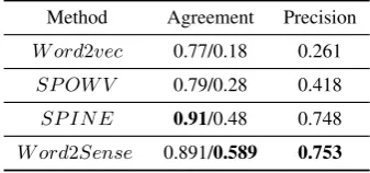
We evaluate the interpretability of the W ord2Sense embeddings against W ord2vec, SP IN E and SP OW V models using the word intrusion test following the procedure in (Subramanian et al., 2018). We select the 15k most frequent words in the intersection of our vocabulary and the Leipzig corpus (Goldhahn et al., 2012). We select a set H of 300 random dimensions or senses from 2250 senses. For each dimension h ∈ H, we sort the words in the 15k vocabulary based on their weight in dimensionh. We pick the top 4 words in the dimension and add to this set a random intruder word that lies in the bottom half of the dimensionhand in the top 10 percentile of some other dimensionh0 ∈H\ {h} (Fyshe et al., 2014; Faruqui et al., 2015). For the dimension h to be claimed interpretable, independent judges must be able to easily separate the intruder word from the top 4 words.
We split the 300 senses into ten sets of 30 senses, and assigned 3 judges to annotate the in-truder in each of the 30 senses in a set (we used a total of 30 judges). For each question, we take the majority voted word as the predicted intruder. If a question has 3 different annotations, we count that dimension as non interpretable6. Since, we
followed the procedure as in (Subramanian et al.,
2018), we compare our performance with the re-sults reported in their paper. Table 5 shows that W ord2Sense is competitive with the best inter-pretable embeddings.
6(Subramanian et al.,2018) used a randomly picked
in-truder in this case.
Method Agreement Precision
W ord2vec 0.77/0.18 0.261
SP OW V 0.79/0.28 0.418
SP IN E 0.91/0.48 0.748
W ord2Sense 0.891/0.589 0.753
Table 5: Comparison of embeddings on for Word Intru-sion tasks. The second column indicates the inter an-notator agreement – the first number is the fraction of questions for which at least 2 annotators agreed and the second indicates the fraction on which all three agreed. The last column is the precision of the majority vote.
6.1 Qualitative evaluation
We show the effectiveness of our embeddings at capturing multiple senses of a polysemous word inTable 1. For e.g. ”tie” can be used as a verb to mean tying a rope, or drawing a match, or as a noun to mean clothing material. These three senses are captured in the top 3 dimensions of W ord2Sense embedding for ”tie”. Similarly, the embedding for ”cell” captures the 5 senses dis-cussed insection 1within the top 15 dimensions of the embedding. The remaining top senses cap-ture fine grained senses such as different kinds of biological cells – e.g. bone marrow cell, liver cell, neuron – that a subject expert might relate to.
7 W ordCtx2Sense embeddings
A word with several senses in the training corpus, when used in a context, would have a narrower set of senses. It is therefore important to be able to refine the representation of a word according to its usage in a context. Note that W ord2vec and W ord2GM models do not have such a mecha-nism. Here, we present an algorithm that gener-ates an embedding for a target wordwˆ in a short context T = {w1, .., wN} that reflects the sense
in which the target word was used in the context. For this, we suppose that the senses of the wordwˆ in contextT are anintersectionof the senses ofwˆ andT. We therefore infer the sense distribution of T by restricting the support of the distribution to those senseswˆcan take.
7.1 Methodology
We suppose that the words in the contextT were picked from a mixture of a small number of senses. Let Sk = {ψ = (ψ1, ψ2, ..., ψk) : ψz ≥
0;P
zψz = 1}be the unit positive simplex. The
generative model is as follows. Pick a ψ ∈ Sk,
the corpus. PickN words fromP independently.
Let A∼P =βψ, ψ∈Sk, (3)
where A is a vocabulary-sized vector containing the count of each word, normalized to sum1. We do not use the Dirichlet prior over sense distribu-tion as in the generative model in section 4, as we found its omission to be better at inferring the sense distribution of contexts.
Given A andβ, we want to infer the sense dis-tributionψ ∈ Sk that minimizes the log
perplex-ity f(ψ;A, β) = −P|V|
i Ailog(βψ)i according
to the generative model inEquation 3. The MWU – multiplicative weight update – algorithm (See
Appendix Afor details) is a natural choice to find such a distributionψ, and has an added advantage. The MWU algorithm’s estimate of a variable ψ w.r.t. a functionf aftertiterations (denotedψ(t))
satisfies
ψ(t)[i] = 0, ifψ(0)[i] = 0∀i∈ {1..k}and∀t≥0.
Therefore, to limit the set of possible senses in the inference of ψ to the µ senses that wˆ can take, we initialize ψ(0) to the embeddingvwˆ. We used
the embedding obtained inEquation 2without the P rojectoperator that adds probabilities of similar senses, to correspond with the use of the original matrixβfor MWU.
Further, to keep iterates close to the initialψ(0),
we add a regularizer to log perplexity. This is necessary to bias the final inference towards the senses that the target word has higher weights on. Thus the loss function on which we run MWU with starting pointψ(0)=vwˆ is
f(ψ;A, β) =−
|V|
X
i=1
Ailog(βψ)i+λKL(ψ, ψ(0))
(4) where the second term is the KL divergence between two distributions scaled by a hy-perparameter λ. Recall that KL(p, q) = −Pk
i=1pilog(pi/qi)for two distributionsp, q ∈ Rk. We use the final estimate ψ(t) as the
Word-Ctx2Sense distribution of a word in the context.
7.2 Evaluation
We demonstrate that the above construction of a word’s representation disambiguated in a context is useful by comparing with state-of-the-art unsu-pervised methods for polysemy disambiguation on two tasks: Word Sense Induction and contextual
similarity. Specifically, we compare with MSSG, theK-Grassmeans model of (Mu et al.,2017), and the sparse coding method of (Arora et al.,2018).7
7.2.1 Hyperparameters
We use the same hyperparameter values forα,β, kandnas insection 5.2.1. We useµ= 100since we do not merge senses in this construction. We tune the hyperparameterλto the task at hand.
7.2.2 Word Sense Induction
The WSI task requires clustering a collection of (say40) short texts, all of which share a common polysemous word, in such a way that each cluster uses the common word in the same sense. Two datasets for this task are Semeval-2010 ( Manand-har et al.,2010) and MakeSense-2016 (Mu et al.,
2017). The evaluation criteria are F-score ( Ar-tiles et al.,2009) and V-Measure (Rosenberg and Hirschberg,2007). V-measure measures the qual-ity of a cluster as the harmonic mean of homo-geneity and coverage, where homohomo-geneity checks if all the data-points that belong to a cluster be-long to the same class and coverage checks if all the data-points of the same class belong to a single cluster. F-score is the harmonic mean of precision and recall on the task of classifying whether the in-stances in a pair belong to the same cluster or not. F-score tends to be higher with a smaller number of clusters and the V-Measure tends to be higher with a larger number of clusters, and it is impor-tant to show performance in both metrics.
For each text corresponding to a polysemous word, we learn a sense distribution ψ using the steps insection 7.1. We tuned the parameterλand found the best performance atλ= 10−2. We use hard decoding to assign a cluster label to each text, i.e., we assign a labelk? = argmaxkψk to a text
with inferred sense vectorψk.
Suppose that this yields ˆk distinct clusters for the instances corresponding to a polysemous word. We cluster them using agglomerative clus-tering into a final set ofK clusters. The distance metric used to group two clustersDiandDjis
d(Di, Dj) =maxa∈Di,b∈Dj(J S[a, b])0.5
7
MakeSense-2016 SemEval-2010
Method K F-scr V-msr F-scr V-msr
(Huang et al.,2012) - 47.40 15.50 38.05 10.60 (Neelakantan et al.,2015)
300D.30K.key - 54.49 19.40 47.26 9.00
300D.6K.key - 57.91 14.40 48.43 6.90
(Mu et al.,2017) 2 64.66 28.80 57.14 7.10
5 58.25 34.30 44.07 14.50
(Arora et al.,2018) 2 - - 58.55 6.1
5 - - 46.38 11.5
W ordCtx2Sense 2 63.71 22.20 59.38 6.80
λ= 0.0 5 59.75 32.90 46.47 13.20
6 59.13 34.20 44.04 14.30
W ordCtx2Sense 2 65.27 24.40 59.15 6.70
λ= 10−2 5 62.88 35.00 47.34 13.70
[image:9.595.71.317.62.259.2]6 61.43 35.30 44.70 15.00
Table 6: Comparison of W ordCtx2Sense with the state-of-the-art methods for Word Sense Induction on MakeSense-2016 and SemEval-2010 dataset. We report F-score and V-measure F-scores multiplied by 100.
Method Pearson-coefficient
W ordCtx2Sense(a) 0.666 W ordCtx2Sense(b) 0.670
W ord2Sense 0.644
W ord2vec 0.651
(Mu et al.,2017) 0.637 (Huang et al.,2012) 0.657 (Arora et al.,2018) 0.652
W ord2GM 0.655
MSSG.300D.30K 0.679a
[image:9.595.332.512.70.193.2]MSSG.300D.6K 0.678a
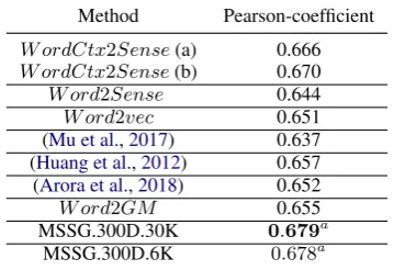
Table 7: Comparison on the SCWS task. Setting (a) forW ordCtx2Sense usesλ = 0.1 for all pairs, and setting (b) usesλ = 10−3 for pairs containing same target words and λ = 0.1 for all other pairs. W ord2Sense,W ord2V ec and W ord2GM neglect context and compare target words.anumbers reported from (Mu et al.,2017) whose experimental setup we could replicate.
where JS is the similarity matrix defined in sec-tion 5.
Results Table 6 shows the results of clus-tering on WSI SemEval-2010 dataset. Word-Ctx2Sense outperforms (Arora et al., 2018) and (Mu et al.,2017) on both F-score and V-measure scores by a considerable margin. We observe simi-lar improvements on the MakeSense-2016 dataset.
7.2.3 Word Similarity in Context
The Stanford Contextual Word Similarity task (Huang et al., 2012) consists of 2000 pairs of words, along with the contexts the words occur in. Ten human raters were asked to rate the similarity of each pair words according to their use in the corresponding contexts, and their average score (on a 1 to 10 scale) is provided as the ground-truth similarity score. The goal of a contextual embed-ding would be to score these examples to maxi-mize the correlation with this ground-truth.
We compute the W ordCtx2Sense of each word in its respective context as in section 7.1. For comparing the meaning of two words in context, we use the JS divergence between their W ordCtx2Sense embeddings. We re-port the coefficient between the ground-truth and W ordCtx2Sense according to two different set-tings ofλ. (a)λ= 0.1, and b)λ= 10−3for
infer-ring the contextual embedding of a word in those pairs that contain same target words, andλ= 0.1 for all other pairs. The main idea is to reduce un-necessary bias for comparing sense of a polyse-mous word in two different contexts.
Results Table 7shows that sense embeddings using context information perform better than all the existing models, except MSSG models ( Nee-lakantan et al.,2015). Also, computing the embed-dings of a word using the contextual information improves results by aprox. 0.025, compared to the case when words embeddings are used directly.
8 Conclusion and future work
We motivated an efficient unsupervised method to embed words, in and out of context, in a way that captures their multiple senses in a corpus in an terpretable manner. We demonstrated that such in-terpretable embeddings can be competitive with dense embeddings like W ord2vec on similarity tasks and can capture entailment effectively. Fur-ther, the construction provides a natural mecha-nism to refine the representation of a word in a short context by disambiguating its senses. We have demonstrated the effectiveness of such con-textual representations.
A natural extension to this work would be to capture the sense distribution of sentences using the same framework. This will make our model more comprehensive by enabling the embedding of words and short texts in the same space.
9 Acknowledgements
References
Sanjeev Arora, Yuanzhi Li, Yingyu Liang, Tengyu Ma, and Andrej Risteski. 2018. Linear algebraic struc-ture of word senses, with applications to polysemy.
Transactions of the Association of Computational Linguistics, 6:483–495.
Javier Artiles, Enrique Amig´o, and Julio Gonzalo. 2009. The role of named entities in web people search. InProceedings of the 2009 Conference on Empirical Methods in Natural Language Process-ing: Volume 2-Volume 2, pages 534–542. Associa-tion for ComputaAssocia-tional Linguistics.
Ben Athiwaratkun and Andrew Gordon Wilson. 2017. Multimodal word distributions. arXiv preprint arXiv:1704.08424.
Marco Baroni, Raffaella Bernardi, Ngoc-Quynh Do, and Chung-chieh Shan. 2012. Entailment above the word level in distributional semantics. In Proceed-ings of the 13th Conference of the European Chap-ter of the Association for Computational Linguistics, pages 23–32. Association for Computational Lin-guistics.
Marco Baroni, Silvia Bernardini, Adriano Ferraresi, and Eros Zanchetta. 2009. The WaCky wide web: a collection of very large linguistically processed web-crawled corpora. Language resources and evaluation, 43(3):209–226.
Samuel Brody and Mirella Lapata. 2009. Bayesian word sense induction. In Proceedings of the 12th Conference of the European Chapter of the Associa-tion for ComputaAssocia-tional Linguistics, pages 103–111. Association for Computational Linguistics.
Elia Bruni, Nam-Khanh Tran, and Marco Baroni. 2014. Multimodal distributional semantics. Journal of Ar-tificial Intelligence Research, 49:1–47.
Eugene Charniak et al. 2013. Naive Bayes word sense induction. InProceedings of the 2013 Conference on Empirical Methods in Natural Language Pro-cessing, pages 1433–1437.
Jianfei Chen, Kaiwei Li, Jun Zhu, and Wenguang Chen. 2016. WarpLDA: a cache efficient O(1) algo-rithm for Latent Dirichlet Allocation. Proceedings of the VLDB Endowment, 9(10):744–755.
Jacob Devlin, Ming-Wei Chang, Kenton Lee, and Kristina Toutanova. 2018. BERT: Pre-training of deep bidirectional transformers for language under-standing. arXiv preprint arXiv:1810.04805.
Paramveer S Dhillon, Dean P Foster, and Lyle H Un-gar. 2015. Eigenwords: Spectral word embed-dings. The Journal of Machine Learning Research, 16(1):3035–3078.
Bhuwan Dhingra, Christopher J Shallue, Mohammad Norouzi, Andrew M Dai, and George E Dahl. 2018. Embedding text in hyperbolic spaces. arXiv preprint arXiv:1806.04313.
Manaal Faruqui, Yulia Tsvetkov, Dani Yogatama, Chris Dyer, and Noah Smith. 2015. Sparse overcom-plete word vector representations. arXiv preprint arXiv:1506.02004.
Lev Finkelstein, Evgeniy Gabrilovich, Yossi Matias, Ehud Rivlin, Zach Solan, Gadi Wolfman, and Ey-tan Ruppin. 2002. Placing search in context: The concept revisited. ACM Transactions on informa-tion systems, 20(1):116–131.
Alona Fyshe, Partha P Talukdar, Brian Murphy, and Tom M Mitchell. 2014. Interpretable semantic vec-tors from a joint model of brain-and text-based meaning. In Proceedings of the conference. Asso-ciation for Computational Linguistics. Meeting, vol-ume 2014, page 489. NIH Public Access.
Dirk Goldhahn, Thomas Eckart, and Uwe Quasthoff. 2012. Building large monolingual dictionaries at the Leipzig corpora collection: From 100 to 200 lan-guages. InLREC, volume 29, pages 31–43.
Weiwei Guo and Mona Diab. 2011. Semantic topic models: Combining word distributional statistics and dictionary definitions. In Proceedings of the Conference on Empirical Methods in Natural Lan-guage Processing, pages 552–561. Association for Computational Linguistics.
Guy Halawi, Gideon Dror, Evgeniy Gabrilovich, and Yehuda Koren. 2012. Large-scale learning of word relatedness with constraints. In Proceedings of the 18th ACM SIGKDD international conference on Knowledge discovery and data mining, pages 1406– 1414. ACM.
Lushan Han, Tim Finin, Paul McNamee, Anupam Joshi, and Yelena Yesha. 2012. Improving word similarity by augmenting PMI with estimates of word polysemy. IEEE Transactions on Knowledge and Data Engineering, 25(6):1307–1322.
Felix Hill, Roi Reichart, and Anna Korhonen. 2015. Simlex-999: Evaluating semantic models with (gen-uine) similarity estimation. Computational Linguis-tics, 41(4):665–695.
Eric H Huang, Richard Socher, Christopher D Man-ning, and Andrew Y Ng. 2012. Improving word representations via global context and multiple word prototypes. InProceedings of the 50th Annual Meet-ing of the Association for Computational LMeet-inguis- Linguis-tics: Long Papers-Volume 1, pages 873–882. Asso-ciation for Computational Linguistics.
Jey Han Lau, Paul Cook, Diana McCarthy, Spandana Gella, and Timothy Baldwin. 2014. Learning word sense distributions, detecting unattested senses and identifying novel senses using topic models. In Pro-ceedings of the 52nd Annual Meeting of the Associa-tion for ComputaAssocia-tional Linguistics (Volume 1: Long Papers), volume 1, pages 259–270.
Jey Han Lau, Paul Cook, Diana McCarthy, David New-man, and Timothy Baldwin. 2012. Word sense in-duction for novel sense detection. In Proceedings of the 13th Conference of the European Chapter of the Association for Computational Linguistics, pages 591–601. Association for Computational Lin-guistics.
Angeliki Lazaridou, Eva Maria Vecchi, and Marco Ba-roni. 2013. Fish transporters and miracle homes: How compositional distributional semantics can help NP parsing. In Proceedings of the 2013 Con-ference on Empirical Methods in Natural Language Processing, pages 1908–1913.
R´emi Lebret and Ronan Collobert. 2013. Word emdeddings through Hellinger PCA. arXiv preprint arXiv:1312.5542.
Omer Levy and Yoav Goldberg. 2014. Neural word embedding as implicit matrix factorization. In Ad-vances in neural information processing systems, pages 2177–2185.
Omer Levy, Yoav Goldberg, and Ido Dagan. 2015. Im-proving distributional similarity with lessons learned from word embeddings. Transactions of the Associ-ation for ComputAssoci-ational Linguistics, 3:211–225.
Xin Li and Dan Roth. 2006. Learning question clas-sifiers: the role of semantic information. Natural Language Engineering, 12(3):229–249.
Thang Luong, Richard Socher, and Christopher Man-ning. 2013. Better word representations with recur-sive neural networks for morphology. In Proceed-ings of the Seventeenth Conference on Computa-tional Natural Language Learning, pages 104–113.
Suresh Manandhar, Ioannis P Klapaftis, Dmitriy Dli-gach, and Sameer S Pradhan. 2010. Semeval-2010 task 14: Word sense induction & disambiguation. InProceedings of the 5th international workshop on semantic evaluation, pages 63–68. Association for Computational Linguistics.
Tomas Mikolov, Ilya Sutskever, Kai Chen, Greg S Cor-rado, and Jeff Dean. 2013. Distributed representa-tions of words and phrases and their compositional-ity. InAdvances in neural information processing systems, pages 3111–3119.
George A Miller and Walter G Charles. 1991. Contex-tual correlates of semantic similarity. Language and cognitive processes, 6(1):1–28.
Jiaqi Mu, Suma Bhat, and Pramod Viswanath. 2017. Geometry of polysemy. In Proceedings of the 5th International Conference on Learning Representa-tions. OpenReview.net.
Brian Murphy, Partha Talukdar, and Tom Mitchell. 2012. Learning effective and interpretable semantic models using non-negative sparse embedding. Pro-ceedings of COLING 2012, pages 1933–1950.
Boris Muzellec and Marco Cuturi. 2018. Generaliz-ing point embeddGeneraliz-ings usGeneraliz-ing the wasserstein space of elliptical distributions. In S. Bengio, H. Wallach, H. Larochelle, K. Grauman, N. Cesa-Bianchi, and R. Garnett, editors,Advances in Neural Information Processing Systems 31, pages 10237–10248. Curran Associates, Inc.
Arvind Neelakantan, Jeevan Shankar, Alexandre Passos, and Andrew McCallum. 2015. Effi-cient non-parametric estimation of multiple embed-dings per word in vector space. arXiv preprint arXiv:1504.06654.
Patrick Pantel and Dekang Lin. 2002. Discovering word senses from text. InProceedings of the eighth ACM SIGKDD international conference on Knowl-edge discovery and data mining, pages 613–619. ACM.
Ted Pedersen. 2000. A simple approach to building en-sembles of Naive Bayesian classifiers for word sense disambiguation. arXiv preprint cs/0005006.
Jeffrey Pennington, Richard Socher, and Christopher Manning. 2014. Glove: Global vectors for word representation. InProceedings of the 2014 confer-ence on empirical methods in natural language pro-cessing (EMNLP), pages 1532–1543.
Matthew E Peters, Mark Neumann, Mohit Iyyer, Matt Gardner, Christopher Clark, Kenton Lee, and Luke Zettlemoyer. 2018. Deep contextualized word rep-resentations. arXiv preprint arXiv:1802.05365.
Kira Radinsky, Eugene Agichtein, Evgeniy Gabrilovich, and Shaul Markovitch. 2011. A word at a time: computing word relatedness using temporal semantic analysis. In Proceedings of the 20th international conference on World wide web, pages 337–346. ACM.
Joseph Reisinger and Raymond J Mooney. 2010. Multi-prototype vector-space models of word mean-ing. InHuman Language Technologies: The 2010 Annual Conference of the North American Chap-ter of the Association for Computational Linguistics, pages 109–117. Association for Computational Lin-guistics.
Herbert Rubenstein and John B Goodenough. 1965. Contextual correlates of synonymy. Communica-tions of the ACM, 8(10):627–633.
Noam Shazeer, Ryan Doherty, Colin Evans, and Chris Waterson. 2016. Swivel: Improving embed-dings by noticing what’s missing. arXiv preprint arXiv:1602.02215.
Richard Socher, Alex Perelygin, Jean Wu, Jason Chuang, Christopher D Manning, Andrew Ng, and Christopher Potts. 2013. Recursive deep models for semantic compositionality over a sentiment tree-bank. In Proceedings of the 2013 conference on empirical methods in natural language processing, pages 1631–1642.
Karl Stratos, Michael Collins, and Daniel Hsu. 2015. Model-based word embeddings from decomposi-tions of count matrices. InProceedings of the 53rd Annual Meeting of the Association for Computa-tional Linguistics and the 7th InternaComputa-tional Joint Conference on Natural Language Processing (Vol-ume 1: Long Papers), volume 1, pages 1282–1291.
Anant Subramanian, Danish Pruthi, Harsh Jhamtani, Taylor Berg-Kirkpatrick, and Eduard Hovy. 2018. Spine: Sparse interpretable neural embeddings. In
Thirty-Second AAAI Conference on Artificial Intelli-gence.
Fei Sun, Jiafeng Guo, Yanyan Lan, Jun Xu, and Xueqi Cheng. 2016. Sparse word embeddings using L1 regularized online learning. In Proceedings of the Twenty-Fifth International Joint Conference on Ar-tificial Intelligence, pages 2915–2921. AAAI Press.
Guoyu Tang, Yunqing Xia, Jun Sun, Min Zhang, and Thomas Fang Zheng. 2014. Topic models incorpo-rating statistical word senses. InInternational Con-ference on Intelligent Text Processing and Computa-tional Linguistics, pages 151–162. Springer.
Guoyu Tang, Yunqing Xia, Jun Sun, Min Zhang, and Thomas Fang Zheng. 2015. Statistical word sense aware topic models.Soft Computing, 19(1):13–27.
Fei Tian, Hanjun Dai, Jiang Bian, Bin Gao, Rui Zhang, Enhong Chen, and Tie-Yan Liu. 2014. A probabilis-tic model for learning multi-prototype word embed-dings. InProceedings of COLING 2014, the 25th In-ternational Conference on Computational Linguis-tics: Technical Papers, pages 151–160.
Alexandru Tifrea, Gary B´ecigneul, and Octavian-Eugen Ganea. 2019. Poincar´e GloVe: Hyperbolic word embeddings. InProceedings of the 7th Inter-national Conference on Learning Representations.
Luke Vilnis and Andrew McCallum. 2015. Word rep-resentations via Gaussian embedding. In Proceed-ings of the 3rd International Conference on Learn-ing Representations.
Jing Wang, Mohit Bansal, Kevin Gimpel, Brian D Ziebart, and Clement T Yu. 2015. A sense-topic model for word sense induction with unsupervised data enrichment. Transactions of the Association for Computational Linguistics, 3:59–71.
Guangxu Xun, Yaliang Li, Jing Gao, and Aidong Zhang. 2017. Collaboratively improving topic dis-covery and word embeddings by coordinating global and local contexts. InProceedings of the 23rd ACM SIGKDD International Conference on Knowledge Discovery and Data Mining, pages 535–543. ACM.
A Multiplicate Weight Update
Algorithm 1Multiplicative Weight update
1: functionMWU(k,Lf, f,θ(0), ITER)
.k denotes dimension of variable θ, f denotes a function of θ, Lf if lipschitz
constant of f,θ0 denotes initial starting point
ofθ, ITER denotes the number of iterations to run
2: fortdo= 1 .. ITER
3: η= 1k p2log(k/t)
4: θˆ(t)=θˆ(t−1)exp (η∇f(θ)|θ=θ(t−1))) 5: θt=θˆ(t)/kθˆ(t)k1
6: end for 7: end function
B Hyper-parameter tuning for W ord2vec
We use the default hyperparameters for training W ord2vec, as given in Mikolov et al. (2013). We tuned the embedding size, to see if the per-formance improves with increasing number of di-mensions. Table 8shows that there is minor im-provement in performance in different similarity and relatedness tasks as the embedding size is in-creased from 100 to 500.
C Hyper-parameter tuning for W ord2GM
We use the default hyperparameters for training W ord2GM, as given inAthiwaratkun and Wilson
(2017). We tuned the embedding size, to see if the performance improves with increasing number of dimensions.Table 9shows that there is minor im-provement in performance of W ord2GM, when the embedding size is increased from 100 to 400.
D Hyper-parameter tuning for W ord2Sense
For generating senses, we use WarpLDA that has 3 different hyperparameters, a) Number of topics kb)α, the dirichlet prior of sense distribution of each word and c)γ, the dirichlet prior of word dis-tribution of each sense. We keepkfixed at 3000 and varyαandβ. We show a small subset of the hyperparameter space searched forα andβ. We report the performance of word embeddings com-puted by Equation 3, without the P roject step, in different similarity tasks. Table 10shows that
the performance slowly decreases as we increase βand somewhat stays constant withα. Hence, we chooseα = 0.1amd γ = 0.001for carrying out our experiments.
E Benchmark downstream tasks
In this section, we discuss about the different downstream tasks considered. We follow the same procedure as (Faruqui et al.,2015) and ( Subrama-nian et al.,2018)8.
• Sentiment analysisThis is a binary classi-fication task on Sentiment Treebank dataset (Socher et al., 2013). The task is to give a sentence a positive or a negative sentiment la-bel. We used the provided train, dev. and test splits of sizes 6920, 872 and 1821 sentences respectively.
• Noun phrase bracketingNP bracketing task (Lazaridou et al., 2013) involves classifying a noun phrase of 3 words as left bracketed or right bracketed. The dataset contains 2,227 noun phrases split into 10 folds. We append the word vectors of three words to get feature representation (Faruqui et al.,2015). We re-port 10-fold cross validation accuracy.
• Question classification Question classifica-tion task (Li and Roth, 2006) involves clas-sifying a question into six different types, e.g., whether the question is about a location, about a person or about some numeric infor-mation. The training dataset consists of 5452 labeled questions, and the test dataset con-sists of 500 questions.
• News classification We consider three bi-nary categorization tasks from the 20 News-groups dataset. Each task involves cate-gorizing a document according to two re-lated categories (a) Sports: baseball vs. hockey (958/239/796) (b) Comp.: IBM vs. Mac (929/239/777) (c) Religion: atheism vs. christian (870/209/717), where the brackets show training/dev./test splits.
8We use the evaluation code given in
Dataset W ord2vec−100 W ord2vec−200 W ord2vec−300 W ord2vec−400 W ord2vec−500
SCWS 0.638 0.646 0.648 0.649 0.651
Simlex-999 0.365 0.388 0.387 0.393 0.393
MEN 0.749 0.760 0.763 0.767 0.780
RW 0.361 0.361 0.363 0.365 0.365
MT-771 0.684 0.685 0.681 0.681 0.688
WS353 0.705 0.719 0.721 0.733 0.732
WS353-S 0.744 0.766 0.768 0.768 0.769
[image:14.595.75.521.67.169.2]WS353-R 0.669 0.679 0.670 0.696 0.703
Table 8: Performance ofW ord2vecat different embedding size, in similarity tasks.
Dataset W ord2GM−100 W ord2GM−200 W ord2GM−400
SL 0.345 0.385 0.398
WS353 0.664 0.672 0.669
WS353-S 0.727 0.735 0.751
WS353-R 0.626 0.625 0.607
MEN 0.740 0.755 0.761
MC 0.812 0.802 0.826
RG 0.730 0.772 0.750
MT-771 0.638 0.664 0.682
[image:14.595.150.446.205.315.2]RW 0.303 0.338 0.338
Table 9: Performance ofW ord2GM, with spherical covariance matrix for each embeddding, at different embed-ding sizes in similarity tasks
α,γ SCWS MT-771 WS353 RG MC WS353-S WS353-R MEN
0.1, 0.001 0.596 0.623 0.654 0.794 0.767 0.685 0.662 0.754
0.1, 0.005 0.595 0.625 0.647 0.809 0.758 0.699 0.638 0.748
0.1, 0.1 0.584 0.609 0.601 0.733 0.671 0.618 0.626 0.738
1.0, 0.001 0.596 0.607 0.651 0.815 0.700 0.692 0.658 0.743
1.0, 0.005 0.613 0.620 0.640 0.792 0.691 0.676 0.653 0.749
1.0, 0.05 0.559 0.562 0.583 0.730 0.742 0.609 0.581 0.711
1.0, 0.1 0.587 0.602 0.602 0.755 0.720 0.641 0.605 0.727
10.0, 0.001 0.595 0.610 0.628 0.822 0.772 0.664 0.639 0.747
10.0, 0.005 0.608 0.635 0.657 0.808 0.826 0.708 0.648 0.739
10.0, 0.05 0.562 0.539 0.544 0.786 0.710 0.573 0.551 0.717
10.0, 0.1 0.573 0.606 0.570 0.773 0.696 0.612 0.593 0.724
Table 10: Performance ofW ord2Sense as computed in eq. 3without theP rojectstep in similarity tasks, at different hyperparameter settings.
Cluster size Top 10 words with the highest probability in the sense’s distribution
6
tennessee, kentucky, alabama, mississippi, georgia, arkansas, nashville, memphis, louisville, atlanta state, idaho, oregon, montana, wisconsin, utah, nevada, wyoming, states, california
illinois, chicago, wisconsin, michigan, milwaukee, rapids, madison, detroit, iowa, grand
19
lol, im, thats, dont, mrplow, yeah, cant, it, ive, ur im, dont, ive, cant, didnt, thats, lol, ur, my, cos my, ve, have, it, me, n’t, ll, just, blog, but
5
lgame, games, adventure, gameplay, 3d, players, play, arcade, of, fun
game, multiplayer, games, gameplay, gaming, xbox, shooter, gamers, mode, halo cheats, mario, super, game, arcade, unlock, mode, nintendo, cheat, bros
7
charlton, striker, midfield, defender, leeds, midfielder, darren, goal, bowyer, danny swansea, derby, leicester, city, wolves, watford, burnley, boss, stoke, swans manager, albion, club, coach, season, football, boss, fa, robson, gary
[image:14.595.118.478.361.493.2] [image:14.595.87.515.552.713.2]