Munich Personal RePEc Archive
Forecasting oil prices
Degiannakis, Stavros and Filis, George
Panteion University of Social and Political Sciences, Panteion
University of Social and Political Sciences
14 March 2018
1
Forecasting oil prices
Stavros Degiannakis1,2 and George Filis1,2,*
1
Department of Economics and Regional Development, Panteion University of Social and Political Sciences, 136 Syggrou Avenue, 17671, Greece.
2
Department of Accounting, Finance and Economics, Bournemouth University, 89 Holdenhurst Road, BH8 8EB, Bournemouth, UK.
*Corresponding author’s email: [email protected]
PLEASE DO NOT USE WITHOUT PERMISSION
Abstract
The paper examines the importance of combining high frequency information,
along with the market fundamentals, in order to gain incremental forecasting accuracy
for oil prices. Inspired by French et al. (1986) and Bollerslev et al. (1988), who
maintain that future asset returns are also influenced by past volatility, we use daily
volatilities and returns from financial and commodity markets to generate real
out-of-sample forecasts for the monthly oil futures prices. Our results convincingly show that
although the oil market fundamentals are useful for long term forecasting horizons,
the combination of the latter with asset realized volatilities, as these are constructed
using ultra-high frequency data, significantly improve oil price forecasts in short-run
horizons. These findings are both statistically and economically significant, as
suggested by several robustness tests.
Keywords: Oil price forecasting, Brent crude oil, intra-day data, MIDAS, EIA forecasts.
2
1. Introduction
The importance of oil price forecasting has been long established in the extant
literature, as well as, in the economic press and policy documents1. The media also provide anecdotal evidence on the macroeconomic effects of the recent oil price
fluctuations2. Overall, the importance of oil price forecasts stems from the fact that they are essential for stakeholders, such as oil-intensive industries, investors, financial
corporations and risk managers, but also for regulators and central banks, in order to
measure financial and economic stability (Elder and Serletis, 2010). Even more, it has
been long established in the literature that oil price changes significantly impact
growth conditions, external balances and price levels, among others (see, inter alia,
Jo, 2014; Natal, 2012; Bachmeier and Cha, 2011; Kilian et al., 2009; Aguiar‐Conraria
and Wen, 2007; Hamilton, 2008a; Backus and Crucini, 2000) and it can also provide
predictive information for economic variables (see, for instance, Ravazzolo and
Rothman, 2013).
Nevertheless, the literature maintains that oil price forecasting could be a
difficult exercise, due to the fact that oil prices exhibit heterogeneous patterns over
time as at different times they are influenced by different fundamental factors, i.e.
demand or supply of oil, oil inventories, etc.
For instance, according to Hamilton (2009a,b) there are periods when the oil
prices are pushed to higher levels due to major oil production disruptions, which were
not accommodated by a similar reduction in oil demand (e.g. during the Yom Kippur
War in 1973, the Iranian revolution in 1978 or the Arab Spring in 2010). On the other
hand, Kilian (2009) maintains that increased precautionary oil demand due to
uncertainty for the future availability of oil leads to higher oil prices. According to
Kilian (2009), the aforementioned uncertainty increases when geopolitical uncertainty
is high (particularly in the Middle-East region).
1
For instance, the IMF (2016) maintains that the recent fall of oil prices create significant deflationary pressures (especially for the oil-importing economies), imposing further constraints to central banks to support growth, given that many countries currently operate in a low interest rate environment. Even more, at the same report the IMF (2016) concludes that “A protracted period of low oil prices could further destabilize the outlook for oil-exporting countries” (p. XVI). ECB (2016), on the other hand,
maintains that “the fiscal situation has become increasingly more challenging in several major oil
producers, particularly those with currency pegs to the US dollar…”, given that “crude oil prices falling well below fiscal breakeven prices…” (p. 2).
2
Barnato (2016), for example, links oil price fluctuations with the quantitative easing in EMU, arguing
that “Given the recent oil price rise, a key question is to what extent the ECB will raise its inflation
projections for 2016-2018 and what this might signal for its QE (quantitative easing) policy after
March 2017.” Similarly, Blas and Kennedy (2016) highlight the concern that the declining energy
3
Even more, the remarkable growth of several emerging economies, and more
prominently this of the Chinese economy, from 2004 to 2007 significantly increased
the oil demand from these countries, while the oil supply did not follow suit, driving
oil prices at unprecedented levels (Hamilton, 2009a,b; Kilian, 2009). Equivalently, the
global economic recession during the Global Financial Crisis of 2007-09 led to the
collapse of the oil prices, as the dramatic reduction of oil demand was not
accompanied by a reduction in the supply of oil.
Other authors also maintain that most of the largest oil price fluctuations since
the early 70s, reflect changes in oil demand. See, for instance, papers by Barsky and
Kilian (2004), Kilian and Murphy (2012, 2014), Lippi and Nobili (2012), Baumeister
and Peersman (2013), Kilian and Hicks (2013), and Kilian and Lee (2014).
Despite the fact that oil market fundamentals have triggered oil price swings, a
recent strand in the literature maintains that the crude oil market has experienced an
increased financialisation since the early 2000 (see, for instance, Büyüksahin and
Robe, 2014; Silvennoinen and Thorp, 2013; Fattouh et al., 2013; Tang and Xiong,
2012), which has created tighter links between the financial and the oil markets. In
particular, Fattouh et al. (2013) argue that the financialisation of the oil market, as this
is documented by the increased participation of hedge funds, pension funds and
insurance companies in the market, has led to its increased comovements with the
financial markets, as well as, other energy-related and non-energy related
commodities. Akram (2009) also maintains that the financialisation of the oil market
is evident due to the increased correlation between oil and foreign exchange returns.
Thus, apart from the fundamentals that could drive oil prices, financial and
commodity markets are expected to impact oil price fluctuations and thus provide
useful information for oil price forecasts.
Nevertheless, the vast majority of the existing literature uses low frequency
data (monthly or quarterly) to forecast monthly or quarterly oil prices, based solely on
oil market fundamentals. As we explain in Section 2, typical efforts to forecast the
price of oil include time-series and structural models, as well as, the no-change
forecasts.
We further maintain, though, that since oil market fundamentals are available
on a monthly frequency, they cannot capture instant developments in the commodities
and financial markets, as well as, in economic conditions at a higher frequency (e.g.
4
are not incorporating this daily information in their oil price forecasts, rendering
important the combination of high frequency information, along with the market
fundamentals, in order to gain significant incremental forecasting ability.
Against this backdrop the aim of this study is twofold. First, we develop a
forecasting framework that takes into consideration the different channels that provide
predictable information to oil prices (i.e. fundamentals, financial markets,
commodities, macroeconomic factors, etc.). Second, we utilise both low and
ultra-high frequency data (tick-by-tick) to forecast monthly oil prices. We maintain that we
generate real out-of-sample forecasts in the sense that at the point that each forecast is
generated, we do not use any unavailable or future information, which would be
impossible for the forecaster to have at her disposal.
To do so, we employ a MIDAS framework, using tick-by-tick financial and
commodities data, which complement the set of the established oil market
fundamental variables. Several studies have provided evidence that the MIDAS
framework has the ability to improve the forecasting accuracy at a low-frequency,
using information from higher-frequency predictors (see, for instance, Andreou et al.,
2013; Clements and Galvao, 2008, 2009; Ghysels and Wright, 2009; Hamilton,
2008b). Needless to mention that in order to allow for meaningful comparisons, we
also consider the existing state-of-the-art forecasting models. Even more, the
forecasting literature has shown that single model predictive accuracy is
time-dependent and thus there might not be a single model that outperforms all others at all
times. Hence, our paper also compares the forecasts from the MIDAS framework
against combined forecasts.
Our findings show that oil market fundamentals are useful in forecasting oil
futures prices in the long run horizons. Nevertheless, we report, for the first time, that
the combination of oil market fundamentals with ultra-high frequency data from
financial, commodity and macroeconomic assets provide significant incremental
predictive gains in monthly oil price forecasts for the short run horizons. In particular,
the daily realized volatilities from the aforementioned assets, and especially from
foreign exchange, reduce the MSPE by almost 36% in 6-months ahead forecasting
horizon, relatively to the no-change forecast. We further show that at least in the
short-run (up-to 3-month horizon) the use of ultra-high frequency data provides gains
in directional accuracy. The results remain robust to several tests, including
5
performance during turbulent oil market periods. The results are also economically
important, as evident by the results of a trading game.
The rest of the paper is structured as follows. Section 2 briefly reviews the
literature. Section 3 provides a detailed description of the data. Section 4 describes the
econometric approach employed in this paper and the forecasting evaluation
techniques. Section 5 analyses the findings of the study. Section 6 includes the
robustness checks, along with the comparison of the results from the forecasting
framework against the U.S. Energy Information Administration (EIA) official
forecasts and Section 7 reports the results from the trading game. Finally, Section 8
concludes the study.
2. Review of the literature
The aim of this section is not to provide an extensive review of the existing
literature but rather to highlight the current state-of-the-art and motivate our approach.
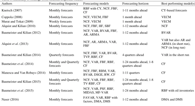
Table 1 provides a summary of the key econometric models that have been used in the
literature, along with their findings.
[TABLE 1 HERE]
One of the early studies in this line of research was conducted by Knetsch
(2007), who uses a random walk and futures-based forecasts as benchmarks and
investigates whether convenience yield forecasting models exhibit a superior
predictive ability. The author considers several definitions for the convenience yield
and finds that the convenience yield forecasting models provide superior forecasts for
1 up to 11 months ahead, as well as, superior prediction of the direction of change,
compared to the two benchmark models.
Coppola (2008) employs Vector Error Correction Models (VECM) using
monthly spot oil prices and a set of futures prices, whereas Murat and Tokat (2009)
employ the same methodology for monthly spot oil prices and crack spread futures.
Both studies show that the VECM model based on the information extracted from the
futures market provide improved forecasts compared to the random walk.
Alquist and Kilian (2010) also focus on the information extracted by the
futures market and forecast monthly oil prices using several specifications of
futures-based models. For robustness, they compare these forecasts against the random walk,
the Hotelling method, as well as, survey-based models. Alquist and Kilian (2010)
6
as their findings suggest that the futures-based forecasts are inferior to the random
walk forecasts.
Furthermore, Baumeister et al. (2013) investigate the usefulness of the product
spot and futures spreads of gasoline and heating oil prices against crude oil prices.
Using several robustness tests, the authors provide evidence that the futures spreads
offer important predictive information of the spot crude oil prices.
Many of the subsequent studies focus on the superior predictive ability of the
VAR-based models. For instance, Baumeister and Kilian (2012) show that recursive
VAR-based forecasts3 based on oil market fundamentals (oil production, oil inventories, global real economic activity) generate lower predictive errors
(particularly at short horizons until 6 months ahead) compared to futures-based
forecasts, as well as, time-series models (AR and ARMA models), and the no-change
forecast. More specifically, the authors use unrestricted VAR, Bayesian VAR
(BVAR) and structural VAR (SVAR) with 12 and 24 lags and their findings suggest
that the BVAR generate both superior forecasts and higher directional accuracy.
Alquist et al. (2013) also suggest that VAR-based forecasts have superior predictive
ability, at least in the short-run, corroborating the results by Baumeister and Kilian
(2012).
Furthermore, Baumeister and Kilian (2014) assess the forecasting ability of a
Time-Varying Parameter (TVP) VAR model, as well as, forecast averaging
techniques. Their findings show that the TVP-VAR is not able to provide better
forecasts compared to the established VAR-based forecasts. Nevertheless, they report
that forecast averaging is capable of improving the VAR-based forecasts, although
only for the longer horizons.
Another study that also provides support to the findings that the VAR-based
models provide superior oil price forecasts is this by Baumeister and Kilian (2016)
who use these models to show the main factors that contributed to the decline in oil
prices from June 2014 until the end of 2014.
Baumeister and Kilian (2015) and Baumeister et al. (2014) extend further this
line of research by examining the advantages of forecast combinations based on a set
of forecasting models, including the no-change and VAR-based forecasts, as well as,
forecasts based on futures oil prices, the price of non-oil industrial raw materials (as
3
7
per Baumeister and Kilian, 2012), the oil inventories and the spread between the
crude oil and gasoline prices. Baumeister and Kilian (2015) also consider a
time-varying regression model using price spreads between crude oil and gasoline prices,
as well as, between crude oil and heating oil prices. Their results show that equally
weighted combinations generate superior predictions and direction of change for all
horizons form 1 to 18 months. These findings remain robust to quarterly forecasts for
up to 6 quarters ahead. Baumeister et al. (2014) further report that higher predictive
accuracy is obtained when forecast combinations are allowed to vary across the
different forecast horizons.
Manescu and Van Robays (2014) further assess the effectiveness of forecast
combinations, although focusing on the Brent crude oil prices, rather than WTI. More
specifically, the authors employ the established oil forecasting frameworks (i.e
variants of VAR, BVAR, future-based and random walk), as well as, a DSGE
framework. The authors provide evidence similar to Baumeister et al. (2014),
showing that none of the competing models is able to outperform all others at all
times and only the forecast combinations are able to constantly generate the most
accurate forecasts for up to 11 months ahead.
More recently, Naser (2016) employs a number of competing models (such as
Autoregressive (AR), VAR, TVP-VAR and FAVAR models) to forecast the monthly
WTI crude oil prices, using data from several macroeconomic, financial and
geographical variables (such as, CPI, oil futures prices, gold prices, OPEC and
non-OPEC oil supply) and compares their predictive accuracy against the Dynamic Model
Averaging (DMA) and Dynamic Model Selection (DMS) approaches. Naser (2016)
finds that the latter approaches exhibit a significantly higher predictive accuracy.
A slightly different approach is adopted by Yin and Yang (2016), who assess
the ability of technical indicators to successfully forecast the monthly WTI prices. In
particular, they use three well-established technical strategies, namely, the moving
average (MA), the momentum (MOM) and on-balance volume averages (VOL),
which are then compared against a series of bivariate predictive regressions. For the
latter regressions the authors use eighteen different macro-financial indicators (such
as, CPI, term spread, dividend yield of the S&P500 index, industrial production, etc.).
Their findings suggest that technical strategies are shown to have superior predictive
8
Thus far we have documented that the VAR-based models seem to exhibit the
highest predictive accuracy both in terms of minimising the forecast error, as well as,
of generating the highest directional accuracy. Even more, there is evidence that
forecast combinations can increase further the predictive accuracy of the VAR-based
models, given that the literature has shown that no single model can outperform all
others over a long time period.
Nevertheless, all aforementioned studies primarily use monthly data not only
for the crude oil prices and the oil market fundamentals but also for all other
macro-financial variables. Baumeister et al. (2015) is the only study to use higher frequency
financial data (weekly4) to forecast the monthly crude oil prices. To do so, authors employ a Mixed-Data Sampling (MIDAS) framework and compare its forecasting
performance against the well-established benchmarks of the no-change and
VAR-based forecasts. Interestingly enough, the authors claim that even though the MIDAS
framework works well, it does not always perform better than the other competing
models and there are cases where it produces forecasts which are inferior to the no-change model. Thus, they maintain that “…not much is lost by ignoring high- frequency financial data in forecasting the monthly real price of oil.” (p. 239).
Contrary to Baumeister et al. (2015) we maintain that the usefulness of
high-frequency financial data in the forecast of oil prices is by no means conclusive. We
make such claim given the compelling evidence that financial markets and the oil
market have shown to exhibit increased comovements over the last decade, as also
aforementioned in Section 1. Furthermore, the use of weekly data may still mask
important daily information which is instrumental to oil price forecasting. We should
not lose sight of the fact that oil prices have exhibited over the last ten years
significant daily variability and so daily data could provide incremental predictive
information. In addition, Baumeister et al. (2015) have not used an exhaustive list of
high-frequency data from financial and commodity markets. Therefore, we maintain
that there is still scope to examine further the benefits of high-frequency financial data
in forecasting oil prices.
4
9
Finally, the bulk literature has concentrated its attention in the forecast of WTI
or the refiner`s acquisition cost of imported crude oil prices, ignoring the importance
of the Brent crude oil price forecasts. In this paper we focus on the latter, which is one
of the main global oil benchmarks, given that a number of institutions, such as the
European Central Bank, the IMF and the Bank of England are primarily interested in
Brent oil price forecasts, rather than WTI (Manescu and Van Robays, 2014).
3. Data Description
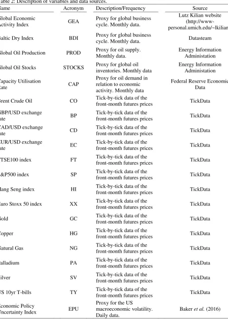
In this study we use both ultra-high and low frequency data. We employ
monthly data for the main oil market fundamentals, as these have been identified by
the literature. In particular, we use the global economic activity index and Baltic Dry
index (as proxies of the global business cycle), the global oil production and the
global oil stocks (as proxies of oil inventories). We also use the capacity utilisation
rate of the oil and gas industry, as an additional measure of oil demand in relation to
economic activity. Kaminska (2009) highlights the link between lower oil prices and
the substantial decrease in oil and refinery capacity utilisation during the global
financial crisis period. The Baltic Dry index, the global oil production and global oil
stocks are converted into their log-returns.
The ultra-high frequency data comprise tick-by-tick prices of the front-month
futures contracts for three major exchange rates (GBP/USD, CAD/USD, EUR/USD),
four stock market indices (FTSE100, S&P500, Hang Seng, Euro Stoxx 50), six
commodities (Brent crude oil, Gold, Copper, Natural Gas, Palladium, Silver) and the
US 10yr T-bills. The tick-by-tick data are used to construct the realized volatilities of
all aforementioned assets5. We also employ the daily US Economic Policy Uncertainty (EPU) index, which, along with the US 10yr T-bills, are proxies of the
global macroeconomic volatility6. In total we consider 15 ultra-high frequency
5
The realized volatility is estimated as the sum of squared intra-day returns and it is adjusted with the close-to-open volatility according to Hansen and Lunde (2005); i.e. minimising the variance of the realized volatility. The intra-day sampling frequency is defined as the highest frequency that minimises the autocovariance bias. More specifically, the intraday sampling frequencies of GBP/USD, CAD/USD and EUR/USD, are 30, 25 and 16 minutes, respectively. The sampling frequencies of FTSE100, S&P500, Hang Seng, Euro Stoxx 50 and US 10y T-bill are 1, 6, 60, 3 and 15 minutes, respectively. Finally, for the commodities, the sampling frequencies of Brent Crude Oil, Gold, Copper, Natural Gas, Palladium and Silver are 23, 15, 20, 10, 90, 28 minutes, respectively.
6
10
series, which belong to four different asset classes, namely, Forex, Stocks,
Commodities and Macro.
The choice of variables is justified by the fact that there is a growing literature
that confirms the cross-market transmission effects between the oil, the commodity
and the financial markets7, as well as, the findings related to the financialisation of the oil market, as discussed in Section 1. For a justification of the specific asset prices,
which are included in our sample, please refer to Degiannakis and Filis (2017).
However, we should also add that the use of exchange rates is also justified by the
claim that when forecasting oil prices for countries other than the United States, the
inclusion of the exchange rates in the forecasting models is necessary (Baumeister and
Kilian, 2014). The specific series are also among the most tradable futures contracts
globally. Furthermore, the aforementioned assets reflect market conditions in Europe,
as well as, globally.
Tick-by-tick data are considered given that we seek to obtain the most
accurate daily information. For instance, Andersen et al. (2006) maintain that
ultra-high frequency data provide the most accurate volatility estimate.
The use of asset returns is motivated by the extant literature which documents spillover effects between oil, commodities and financial assets’ returns, as discussed in Sections 1 and 2. On the other hand, the use of realized volatilities as predictors of
oil prices is related to the arguments put forward by French et al. (1986), Engle et al.
(1987), Bollerslev et al. (1988), among others, that expectations related to future asset
returns are also influenced by its own current and past variance. Hence, motivated by
this argument, we extend it further to assess whether future oil prices are not only
influenced by its own current and past variance, but also by the current and past
variances of other assets.
The period of our study spans from August 2003 to August 2015 and it is
dictated by the availability of intraday data for the Brent Crude oil futures contracts.
Table 2 summarizes the data and the sources from which they have been obtained.
[TABLE 2 HERE]
expire in future years. The third component uses disagreement among economic forecasters as a proxy for uncertainty. For more information the reader is directed to http://www.policyuncertainty.com.
7
See, inter alia, Aloui and Jammazi (2009), Kilian and Park (2009), Sari et al. (2010), Arouri et al.
11
4. Forecasting models
4.1. MIDAS regression model
We define the oil futures price returns at a monthly frequency as
( ⁄ ), and the vector of explanatory variables at a monthly frequency as
( ( ⁄ ) ( ⁄ ) ) , where
, , and denote the global economic activity, the global oil production, the global oil stocks and the capacity utilisation rate, respectively. The
vector of daily returns or realized volatilities is denoted as ( ) ( ) , where is the
number of daily observations at each month. The MIDAS model with polynomial
distributed lag weighting, first proposed by Almon (1965), is expressed as:
∑ ( ) ( ) (∑
)
(1)
where ( ), and , are vectors of coefficients to be estimated. The is
the dimension of the lag polynomial in the vector parameters . The is the number
of lagged days to use, which can be less than or greater than .
The proposed MIDAS model relates the current’s month oil futures price with
the low-frequency explanatory variables months before and the ultra-high frequency
explanatory variables trading days before. Hence, such a model is able to
provide months-ahead oil futures price forecasts. For example, if we intend to
predict the one-month ahead oil price then the MIDAS model is estimated for ,
thus . In the case we intend to predict the three-month ahead oil price then the
MIDAS model is estimated for , so .
The number of lagged days is defined for the minimum sum of squared
residuals, so that at each model’s estimation the optimum varies8. In order to investigate the adequate number of polynomial order, we run a series of model
estimations for various values of . We conclude that the appropriate dimension of
the lag polynomial is .
Denoting the constructed variable based on the lag polynomial as ̃
∑ ( ) ( )
, the MIDAS model is written as:
∑ ̃ . (2)
8
12
The number of vector coefficients to be estimated depends on and not on
the number of daily lags
Technical information for MIDAS model is available in Andreou et al. (2010,
2013). Ghysels et al. (2006, 2007) proposed the weighting scheme to be given by the
exponential Almon lag polynomial or the Beta weighting. Foroni et al. (2015)
proposed the unrestricted MIDAS polynomial. Those polynomial specifications work
adequately for small values of .
In total we estimate 29 MIDAS models, using one asset’s volatility or return at
a time9. We denoted MIDAS-RV and MIDAS-RET the MIDAS models based on realized volatilities and returns, respectively. We should also highlight here that we
have experimented using the daily squared returns as an additional measure of daily
volatility, yet in such case the MIDAS-RV models did not perform satisfactorily.
Hence, our analysis is based on the ultra-high frequency data10.
MIDAS forecasts are compared with the models that have been suggested by
the literature (denoted as the standard models). In particular, we use a random-walk
model (as the no-change forecast), AR(1), AR(12), AR(24) and ARMA(1,1) models,
as well as, VAR-based models. For the latter we use unrestricted VAR models and
BVAR models, with three and four endogenous variables. The trivariate VAR models
include the changes in the global oil production, the global economic activity index
and the Brent crude oil prices, whereas for the four variable VAR models we add the
changes in global oil stocks. We should emphasize here that we estimate the VAR
models using the level oil prices with 12 and 24 lags. The choice of the
aforementioned models is motivated by Baumeister et al. (2015), Kilian and Murphy
(2014) and Baumeister and Kilian (2012), among others.
4.2. Forecast prediction and evaluation
Our forecasts are estimated recursively using an initial sample period of 100
months11. The MIDAS predictions are estimated as in eq. 3:
9
Even though we have 15 assets, EPU is considered as a proxy of macroeconomic volatility and thus it is only included in the set of asset volatilities.
10
Thus, we claim that it is not just the MIDAS model but also the use of tick-by-tick data that are required to produce superior forecasts.
11
13
( ( ) ∑ ( ) ( ) (∑ ( )
)
⁄ ̂ )
(3)
For a description of the competing models’ predictions, please refer to
Baumeister et al. (2015), Kilian and Murphy (2014) and Baumeister and Kilian
(2012).
Initially, the monthly forecasting ability of our models is gauged using both
the Mean Squared Predicted Error (MSPE) and the Mean Absolute Percentage
Predicted Error (MAPPE), relative to the same loss functions of the monthly
no-change forecast. All evaluations are taking place based on the level oil prices. A ratio
above one suggests that a forecasting model is not able to perform better than the
no-change forecast, whereas the reverse holds true for ratios below 1.
To establish further the forecasting performance of the competing models, we
employ the Model Confidence Set (MCS) of Hansen et al. (2011), which identifies
the set of the best models which have equal predictive accuracy, according to a loss
function. The benefit of the MCS test, relative to other approaches (such as the
Diebold Mariano test) is that there is no need for an a priori choice of a benchmark
model12. The MCS test is estimated based on the two aforementioned loss functions. For denoting the initial set of forecasting models, let be the evaluation
function of any model at month t. We denote the evaluation differential as
, for . The is the evaluation function under consideration;
e.g. for the MSPE, we have ( ) , where is the
s-months-ahead oil price forecast. The null hypothesis ( ) , for
, is tested against the ( ) , for some . We also assess the directional accuracy of our models, using the success ratio,
which depicts the number of times a forecasting model is able to predict correctly
whether the oil price will increase or decrease. A ratio below 0.5 denotes no
period. Initial in-sample estimation periods of 90 and 80 months were also considered and the results were qualitatively similar.
12
14
directional accuracy, whereas any values above 0.5 suggest an improvement relatively
to the no-change forecast. We use the Pesaran and Timmermann (2009) test to assess
the significance of the directional accuracy improvements of any model relative to the
no-change forecast.
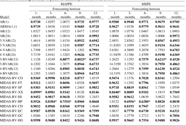
5. Empirical results 5.1. MIDAS-RV models
We start our analysis with the MIDAS-RV and the results are reported in
Table 3. It is evident from Table 3 that almost all MIDAS-RV models exhibit
important gains in forecasting accuracy relatively to the no-change forecast,
suggesting that the financial assets’ volatilities have significant predictive information
for the monthly oil prices. Even more, these gains seem to become quite substantial as
the forecasting horizon increases, although this does not hold for all assets. The fact
that the forecasting gains, relatively to the no-change forecast, increase as the
forecasting horizons extends further out is also observed in Baumeister et al. (2015).
Specifically, we report gains up to about 68% with the MIDAS-RV model, based on
the MPSE in the 12-months-ahead horizon, whereas in the short-run horizons of 1-
and 3-months ahead, the predictive gains are 15% and 30%, respectively.
[TABLE 3 HERE]
Comparing the MIDAS-RV models performance against all other benchmarks
we are able to deduct the conclusion that the former are clearly outperforming. The
only exception is the 9-months ahead forecasting horizon where the trivariate BVAR
model with 12 lags (3-BVAR(12)) outperforms all others, with predictive gains
relatively to the no-change forecast of 38%. We should not lose sight of the fact
though, that even in the 9-month horizon, the MIDAS-RV models generate substantial
predictive gains which reach the level of 20%.
Nevertheless, we observe that at least in the short- and medium-run (up to
6-months horizon), the standard models do not seem to provide any gains in forecasting
accuracy relatively to the no-change forecasts, as opposed to the models that
incorporate the ultra-high frequency based realized volatilities.
It is also important to highlight the fact that, as we move further out to the
forecasting horizon, it is a different asset class that provides the highest forecast
accuracy. More specifically, in the short-run (1-month ahead) the stock market
15
gains. In the medium-run (3- and 6-months ahead) the information obtained from the
foreign exchange market (GBP/USD volatility) enhances the forecasting accuracy of
oil prices, whereas in the long-run we observe that the commodities are assuming the
role of the best performing model (PA volatility). This is a very important finding,
which has not been previous reported in the literature, and suggests that different
assets provide different predictive information for oil prices at the different
forecasting horizons.
Given that Brent crude oil is the benchmark used in the European market, the
fact that the assets which provide the most valuable predictive information are the
Eurostoxx 50 and the GBP/USD volatilities, suggests it is the European rather than
the global financial conditions that incorporate important information for the future
path of oil prices. Even more, we would anticipate that stock market and foreign
exchange volatility would transmit predictive information for oil prices in the short-
and medium-run respectively, given that these markets are more short-run oriented.
By contrast, the longer run predictive information that is contained in palladium
volatility is possibly explained by the fact that this particular commodity is heavily
used by the automobile industry. The latter is an industry tightly linked with
information related to longer run economic prospects. .
Next, we need to establish whether the gains in the forecasting accuracy that
were achieved using the MIDAS-RV models are statistically significantly higher
compared to all other models. To do so, we perform the MCS test, which assesses the
models that can be included among the set of the best performing models with equal
predictive accuracy. The models that are included in the set of the best performing
models are shown in Table 3 with an asterisk.
The MCS test clearly shows that the best performing models in all forecasting
horizons (apart from the 9-month ahead) are the MIDAS-RV models and particularly
the MIDAS-RV-XX, MIDAS-RV-BP and MIDAS-RV-PA. This finding is rather
important as it reinforces our argument that ultra-high frequency data are capable of
providing superior predictive accuracy not only relatively to the no-change forecast,
but also to the current state-of-the-art models.
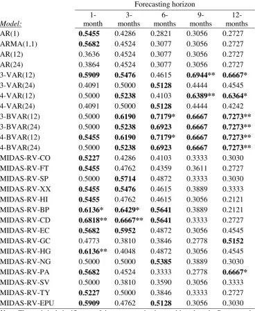
Furthermore, we report the success ratios of the competing models (see Table
4). Our findings suggest that the MIDAS-RV models exhibit high directional
accuracy, which is particularly evident in the shorter horizons (up to 6-months
16
horizon and the MIDAS-RV model. Even more, we show that the MIDAS-RV models
with the exchange rate (i.e. MIDAS-RV-BP and MIDAS-RV-CD) are particularly
those with the highest significance up to 3-months ahead forecasting horizon, along
with the MIDAS-RV-HG. Nevertheless, in the longer term periods we notice that the
VAR and BVAR models exhibit higher success ratios compared to the MIDAS-RV
models. The only exception is the MIDAS-RV-PA which demonstrates significant
success ration in the 12-months ahead horizon.
[TABLE 4 HERE]
5.2. MIDAS-RET models
We proceed further with the examination of whether we can achieve even
higher predictive accuracy using asset returns, as opposed to asset volatilities, based
on the ultra-high frequency data. The results are shown in Table 5.
[TABLE 5 HERE]
Overall, the results suggest that most MIDAS-RET models are not able to
outperform the no-change forecast, constantly, as in most cases the ratios of the loss
functions are above 1. Even more, in the cases where MIDAS-RET models provide
predictive gains, these are not material. Furthermore, the MIDAS-RET models do not
seem to provide any incremental predictive gains compared to the MIDAS-RV
models, suggesting that the main predictive information is transmitted to oil prices via
the uncertainty that exists in the financial, commodities and macroeconomic assets.
The only exception is the MIDAS-RET-CD, which provides important predictive
gains in two horizons (3- and 12-months ahead), classifying it among the set of the
best performing models (based on the MCS test).
Turning our attention to the directional accuracy of the MIDAS-RET models,
we show that even though they improve the directional accuracy of the no-change
forecast, they are able to do so only in the short- to medium-run (i.e. up to the
3-month horizon), as reported in Table 6. Nevertheless, this improvement is not higher
compared to the MIDAS-RV models, providing further evidence of the superior
performance of the latter models compared to MIDAS-RET.
[TABLE 6 HERE]
Section 5 provides convincing empirical evidence that the realized volatility
measures, based on the ultra-high frequency data, provide the more accurate
17
5.3. Predictive accuracy during the oil price collapse of 2014-2015
So far we have shown quite convincingly that MIDAS-RV models can provide
significant gains on both the forecasting and directional accuracy, not only compared
to the no-change forecast but also compared to the current state-of-the-art, as well as
the MIDAS-RET models. This is a rather important finding, which highlights the
importance of the information that can be extracted from the ultra-high frequency
financial and commodities data in forecasting monthly oil prices.
Nevertheless, our out-of-sample forecasting period includes the 2014-15
period that Brent crude oil sharply lost more than 50% of its price. Baumeister and
Kilian (2016) provide a very good overview of the main consequences of this oil price
collapse and the factors that might have contributed to this fall. Oil market
stakeholders are primarily interested in successful oil price predictions during oil
market volatile periods, given that these are the periods that call for actions to
mitigate the adverse effects of sharp oil price changes.
Therefore, motivated by this extreme movement in oil prices between June
2014 and August 2015, coupled with the fact that forecasting instability is a common
problem in forecasting, our next step is to assess the forecasting accuracy of our
MIDAS-RV and MIDAS-RET models, relatively to the standard models in the
literature, during this oil collapse period. The results are shown in Table 7.
[TABLE 7 HERE]
The results from Table 7 are rather interesting, as they clearly show that the
several MIDAS-RV and MIDAS-RET models generate forecasts with the highest
predictive accuracy, relative to the no-change forecast. Importantly, we should
highlight the fact that during this turbulent period, MIDAS-RV models achieve
forecasting gains at the 6-month horizon, which exceed the 60% level (based on the
MSPE). Furthermore, MIDAS-RV models can also provide significant predictive
gains even for the longer run forecasting horizons (9- and 12-months ahead) that
exceed the level of 73% (see MSPE of the MIDAS-PA in the 12-months ahead),
although these gains are relatively lower compared to the predictive gains of the
trivariate and four-variable BVAR(24) models that exceed the level of 81% in the
12-months ahead. The MIDAS-RET models perform better compared to the full
out-of-sample period, nevertheless, they do not outperform the MIDAS-RV models.
In terms of the models that belong to the set with the best performing models
18
horizon, although the MIDAS-RET models with the commodities are also included in
the best performing models at the 1-month horizon.
Overall, we maintain that MIDAS models using ultra-high frequency data are
useful alternatives (especially for the short- to medium-run forecasting horizons) to
the standard models that are currently employed in the literature, although this
primarily holds for the use of realized volatilities rather than the returns.
We should of course highlight here that the findings for the oil collapse period
should be treated as indicative due to the small number of the out-of-sample
observations.
6. Robustness
6.1. MIDAS models based on asset classes’ returns and volatilities.
Next, we investigate whether combined information, either from single asset
classes or from all assets together, we can increase further the forecasting accuracy of
oil prices.
In order to avoid imposing selection and look-ahead bias, we employ the
Principal Component Analysis (PCA) that captures the combined asset class volatility
(return); see for more information Degiannakis and Filis (2017) and Giannone et al.
(2008). For g denoting the number of asset volatilities (returns) within an asset class,
the PCA volatility (returns) components are computed as:
( )
( ) ( ) ( )
( ) ( ) (4)
where ( ) is the matrix of factor loadings, ( ) ( ) is the vector with the common
factors, and ( ) is the vector of the idiosyncratic component. E.g. for the Stocks asset
class, we use the volatilities of the g=4 stock market indices to estimate the PCA
volatility (return) components; ( ) ( ) [
( ) ( )
( ) ( )
], where ( ) denotes the daily
common factors that are incorporated in the MIDAS-RV-Stocks (or
MIDAS-RET-Stocks) models13. We apply the same procedure for the remaining three asset classes.
13
For the returns of the stock market indices, we estimate the PCA return components, ( ) ( )
[ ( ) ( )
( ) ( )
19 Finally, based on PCA we extract the common factors of all assets’ returns or volatilities together, denoted as MIDAS-RV-Combined and MIDAS-RET-Combined.
The results are presented in Tables 8 and 9 for the full out-of-sample period and the
oil collapse period, respectively.
[TABLE 8 HERE]
[TABLE 9 HERE]
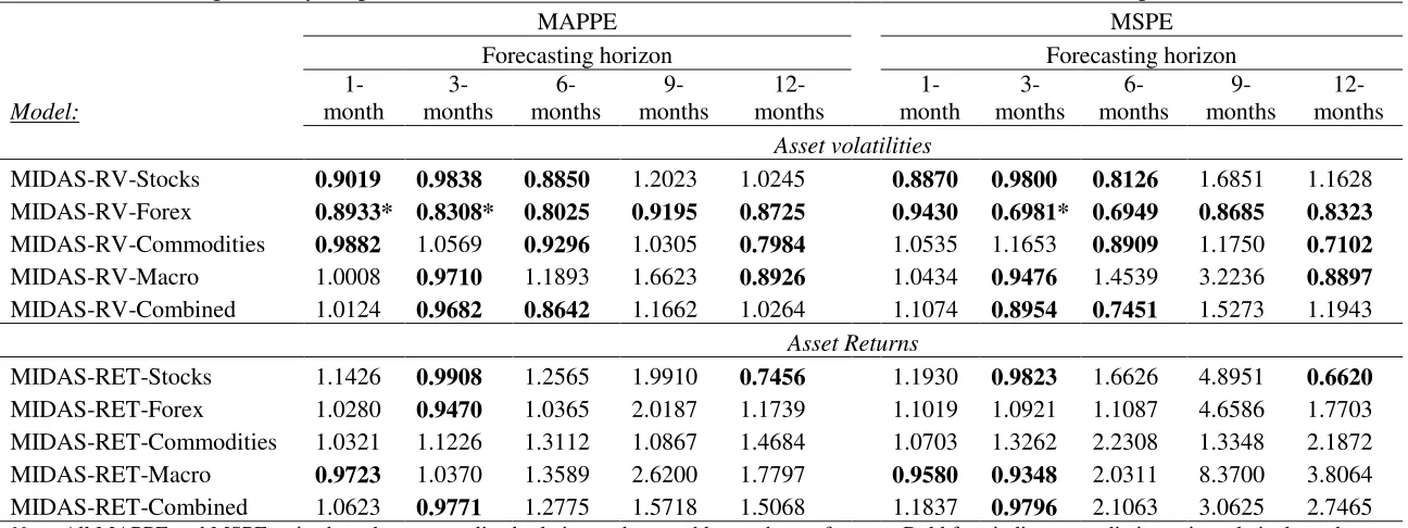
Tables 8 and 9 reveal that even though some of the combined asset classes’
volatilities (e.g. the MIDAS-RV-Forex and MIDAS-RV-Stocks) provide predictive
gains relatively to the no-change forecast in almost forecast horizons, they cannot
outperform the forecasting accuracy of the MIDAS-RV models with single asset
volatility, as shown in Tables 3 and 7. This also holds true for the MIDAS-RET
models. These results also apply for the MIDAS-RV-Combined and
MIDAS-RET-Combined, suggesting that we cannot improve further the forecasting accuracy of oil
prices by combining all assets’ volatilities or returns together.
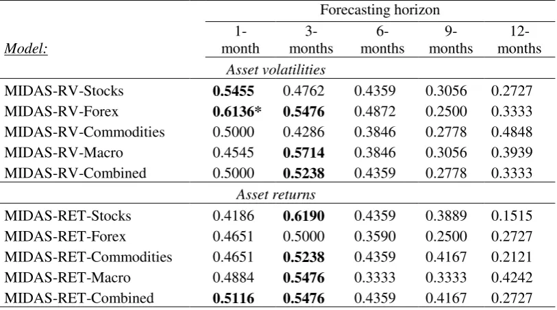
Similar conclusions can be drawn for the directional accuracy of the MIDAS
models based on the four asset classes (see Table 10).
[TABLE 10 HERE]
6.2. Forecast combinations
Finally, we examine whether forecast combinations are able to outperform the
MIDAS-RV models, which are the best performing models thus far. To do so, we
construct three simple average models, namely, the simple average of all standard
models suggested by the literature (denoted as FC-Standard), the simple average of all
MIDAS-RV and MIDAS-RET models, separately (denoted as FC-MIDAS-RV and
FC-MIDAS-RET), and finally the simple average of all competing models (denoted
as FC-All)14. The results are reported in Table 11, whereas, Table 12 exhibits the directional accuracy of the forecast combinations.
[TABLE 11 HERE]
[TABLE 12 HERE]
It is evident from Table 11 that forecast combinations, either in the full
out-of-sample period or in the oil collapse period, are able to perform better than the
14
20
change forecast, nevertheless they cannot provide incremental gains relatively to the
best MIDAS-RV models that were identified in Tables 3 and 7. In terms of directional
accuracy, we show that forecast combinations do not demonstrate improved
directional accuracy.
Overall, the robustness tests confirm our earlier evidence that asset volatilities,
which are constructed using ultra-high frequency data, provide significantly superior
predictive accuracy, as well as, directional accuracy for the monthly oil prices, which
is particularly evident in the shorter run horizons (i.e. up to 3-months ahead).
6.3. Comparing MIDAS-RV forecasts against EIA official forecasts
Next, we proceed with a direct comparison between the forecasts from our
MIDAS-RV models and the EIA’s official forecasts15. The comparisons for the full out-of-sample period and the oil price collapse period are shown in Tables 13 and 14,
respectively.
[TABLE 13 HERE]
[TABLE 14 HERE]
It is evident that the MIDAS-RV models are able to outperform the EIA’s
forecasts in many instances. More importantly, we should highlight that the predictive
gains of the MIDAS-RV models relatively to the EIA’s forecasts can reach up to the
levels of 24% and 42% during the full out-of-sample and oil price collapse period,
respectively (the Figures refer to the 12-months ahead horizon, based on the MSPE
loss function).
Furthermore, we evaluate the incremental directional accuracy of our MIDAS-RV models relatively to directional accuracy of the EIA’s forecasts (see Table 15).
[TABLE 15 HERE]
Even in this case, the MIDAS-RV models seem to be capable of performing better that the EIA’s success ratio, particularly in the short run horizons and for the MIDAS-RV models with the exchange rates (i.e. BP and
MIDAS-RV-CD). Overall, these results highlight further the previous conclusions, i.e. that asset
volatilities provide important superior predictive ability even relatively to the EIA.
15
21
7. Forecast evaluation based on a trading strategy
In this section we compare the trading performance of the standard models of
the literature against the MIDAS-RV models. We proceed to the evaluation of our
forecasts based on a simple trading game so to demonstrate the economic importance
of the forecasting gains from the MIDAS-RV models.
Our trading strategy is as follows. A trader assumes a long (short) position in
the oil futures prices when the t h forecasted oil price is higher (lower) compared to
the actual price at month, t. Cumulative portfolio returns are then calculated as the
aggregate returns over the investment horizon, which equals our out-of-sample
forecasting period, i.e. December, 2011 up to August, 2015. We also calculate the
cumulative returns in dollar terms. Given that the MIDAS-RV models provide
predictive gains and high directional accuracy particularly in the short run horizons,
we present the trading gains/losses for the 1- and 3-months ahead horizons. The
results of the trading strategy are reported in Table 16. The trading game provides
evidence that the MIDAS-RV models constantly generate positive returns, which is
not the case for the standard models. In addition, for the 1-month ahead horizon, the
MIDAS-RV-CD provides the higher positive returns, whereas for the 3-month ahead,
we observe that the 3-BVAR(12) and 4-BVAR(12) models exhibit the highest returns.
Overall, the findings from the trading game confirm the superiority of the
MIDAS-RV models in the short run horizons.
[TABLE 16 HERE]
8. Conclusion
The aim of this study is to forecast the monthly oil futures prices using
information for ultra-high frequency data of financial, commodities and
macroeconomic assets. We do so using a MIDAS model and by constructing daily
realized volatilities from the ultra-high frequency data. Our data span from August
2003 to August 2015. The out-of-sample period runs from December 2011 to August
2015. In our study, real out-of-sample forecasts are generated, i.e. we do not use any
future information, which would be impossible for the forecaster to have at her
disposal at the time that of the forecast.
We compare the forecasts generated by our MIDAS-RV and MIDAS-RET
22
forecasting models. The findings of the study show that for longer term forecasts the
BVAR models tend to exhibit higher predictive accuracy, given that these models are
based on oil market fundamentals, capturing the long term equilibrium relationship
among the global business cycle, global oil production and global oil stocks.
Nevertheless, we show that MIDAS models which combine oil market fundamentals
along with the information flows from the financial markets at a higher sampling
frequency provide superior predictive ability for short-run forecasting horizons (up to
6-months). In particular, the MIDAS models’ predictive gains, relatively to the
no-change forecast, exceed the level of 32% at the 6-month ahead forecasting horizon.
These results hold true even when we only consider the predictive accuracy of our
models during the oil price collapse period of 2014-2015.
For robustness purposes we estimate MIDAS models based on asset classes’
volatilities and returns. The findings confirm that the aggregated information from the
asset classes cannot provide incremental superior predictive accuracy relatively to the
MIDAS-RV models. These results remain robust even when forecast averaging is
employed and when our forecasts are compared against the EIA’s official forecasts.
The results from the trading game also demonstrate that the forecasting gains from
using ultra-high frequency data are economically important.
Hence, we maintain that the use of ultra-high frequency data is able to
significantly enhance the predictive accuracy of the monthly oil price for short run
horizons. Hence, there is still scope to extend further this line of research. For
instance, future research could further investigate the usefulness of ultra-high
frequency data in forecasting oil prices using financial instruments that approximate
aggregated asset classes, such as the US equity index futures, USD index futures and
the S&P-GSCI futures. Future studies should assess how to use the incremental
predictive accuracy of the ultra-high frequency information, which is particularly
obtained in the short run horizons, so to obtain higher forecasting accuracy in longer
23
Acknowledgements
The authors acknowledge the support of the European Union's Horizon 2020
research and innovation programme, which has funded them under the Marie
Sklodowska-Curie grant agreement No 658494. We also thank Lutz Kilian, Vipin
Arora and David Broadstock for their valuable comments on an earlier version of the
paper. Finally, we would also like to thank the participants of the ISEFI 2017
conference, as well as the participants of the research seminars at the Hong Kong
Polytechnic University.
References
Aguiar‐Conraria, L. U. Í. S., & Wen, Y. (2007). Understanding the large negative impact of oil shocks. Journal of Money, Credit and Banking, 39(4), 925-944. Akram, Q. F. (2009). Commodity prices, interest rates and the dollar. Energy
Economics, 31(6), 838-851.
Aloui, C., & Jammazi, R. (2009). The effects of crude oil shocks on stock market shifts behaviour: A regime switching approach. Energy Economics, 31(5), 789-799.
Alquist, R., & Kilian, L. (2010). What do we learn from the price of crude oil futures?. Journal of Applied Econometrics, 25(4), 539-573.
Alquist, R., Kilian, L., & Vigfusson, R. J. (2013). Forecasting the price of oil.
Handbook of Economic Forecasting, 2, 427-507.
Almon, S. (1965). The distributed lag between capital appropriations and expenditures. Econometrica: Journal of the Econometric Society, 178-196. Andreou, E., Ghysels, E., & Kourtellos, A. (2010). Regression models with mixed
sampling frequencies. Journal of Econometrics, 158(2), 246-261.
Andreou, E., Ghysels, E., & Kourtellos, A. (2013). Should macroeconomic forecasters use daily financial data and how?. Journal of Business & Economic Statistics, 31(2), 240-251.
Antonakakis, N., Chatziantoniou, I., & Filis, G. (2014). Dynamic spillovers of oil price shocks and economic policy uncertainty. Energy Economics, 44, 433-447. Arouri, M. E. H., Jouini, J., & Nguyen, D. K. (2011). Volatility spillovers between oil
prices and stock sector returns: implications for portfolio management. Journal of International Money and Finance, 30(7), 1387-1405.
Bachmeier, L. J., & Cha, I. (2011). Why don’t oil shocks cause inflation? Evidence from disaggregate inflation data. Journal of Money, Credit and Banking, 43(6), 1165-1183.
Backus, D. K., & Crucini, M. J. (2000). Oil prices and the terms of trade. Journal of International Economics, 50(1), 185-213.
Baker, S. R., Bloom, N., & Davis, S. J. (2016). Measuring economic policy uncertainty. The Quarterly Journal of Economics, 131(4), 1593-1636.
Barnato, K. (2016). Here’s the key challenge Draghi will face at this week’s ECB meeting, CNBC, 30th May, http://www.cnbc.com/2016/05/30/heres-the-key-challenge-draghi-will-face-at-this-weeks-ecb-meeting.html
24
Baumeister, C., & Kilian, L. (2012). Real-time forecasts of the real price of oil.
Journal of Business & Economic Statistics, 30(2), 326-336.
Baumeister, C., Kilian, L., & Zhou, X. (2013). Are product spreads useful for forecasting? An empirical evaluation of the Verleger hypothesis (No. 2013-25). Bank of Canada Working Paper.
Baumeister, C., & Kilian, L. (2014). What central bankers need to know about forecasting oil prices. International Economic Review, 55(3), 869-889.
Baumeister, C., & Kilian, L. (2015). Forecasting the real price of oil in a changing world: a forecast combination approach. Journal of Business & Economic Statistics, 33(3), 338-351.
Baumeister, C., & Kilian, L. (2016). Understanding the Decline in the Price of Oil since June 2014. Journal of the Association of Environmental and Resource Economists, 3(1), 131-158.
Baumeister, C., Kilian, L., & Lee, T. K. (2014). Are there gains from pooling real-time oil price forecasts?. Energy Economics, 46, S33-S43.
Baumeister, C., Guérin, P., & Kilian, L. (2015). Do high-frequency financial data help forecast oil prices? The MIDAS touch at work. International Journal of Forecasting, 31(2), 238-252.
Baumeister, C., & Peersman, G. (2013). Time-varying effects of oil supply shocks on the US economy. American Economic Journal: Macroeconomics, 5(4), 1-28. Blas, J., & Kennedy, S. (2016). For Once, Low Oil Prices May Be a Problem for
World's Economy, Bloomberg, 2nd February,
https://www.bloomberg.com/news/articles/2016-02-02/for-once-low-oil-prices-may-be-a-problem-for-world-s-economy.
Bollerslev, T., Engle, R. F., & Wooldridge, J. M. (1988). A capital asset pricing model with time-varying covariances. Journal of Political Economy, 96(1), 116-131.
Büyükşahin, B., & Robe, M. A. (2014). Speculators, commodities and cross-market linkages. Journal of International Money and Finance, 42, 38-70.
Clark, T.E., & West, K.D. (2007). Approximately normal tests for equal predictive accuracy in nested models. Journal of Econometrics, 138, 291–311.
Clements, M. P., & Galvão, A. B. (2008). Macroeconomic forecasting with mixed -frequency data: Forecasting output growth in the United States. Journal of Business & Economic Statistics, 26(4), 546-554.
Clements, M. P., & Galvão, A. B. (2009). Forecasting US output growth using leading indicators: An appraisal using MIDAS models. Journal of Applied Econometrics, 24(7), 1187-1206.
Coppola, A. (2008). Forecasting oil price movements: Exploiting the information in the futures market. Journal of Futures Markets, 28(1), 34-56.
Degiannakis, S. & Filis, G. (2017). Forecasting oil price realized volatility using information channels from other asset classes, Journal of International Money and Finance, 76, 28-49.
Diebold, F. X., & Mariano, R. S. (1995). Comparing predictive accuracy. Journal of Business & Economic Statistics, 13, 253-263.
ECB (2016). Economic Bulletin, Issue 4, European Central Bank. https://www.ecb.europa.eu/pub/pdf/other/eb201604_focus01.en.pdf?48284774d 83e30563e8f5c9a50cd0ea2.
25
Engle, R. F., Lilien, D. M., & Robins, R. P. (1987). Estimating time varying risk premia in the term structure: the ARCH-M model. Econometrica, 391-407. Fattouh, B., Kilian, L., & Mahadeva, L. (2013). The Role of Speculation in Oil
Markets: What Have We Learned So Far?. The Energy Journal, 34(3), 7.
French, K. R., Schwert, G. W., & Stambaugh, R. F. (1987). Expected stock returns and volatility. Journal of Financial Economics, 19(1), 3-29.
Foroni, C., Marcellino, M., & Schumacher, C. (2015). Unrestricted mixed data sampling (MIDAS): MIDAS regressions with unrestricted lag polynomials.
Journal of the Royal Statistical Society: Series A, 178(1), 57-82.
Giannone, D., L. Reichlin and D. Small (2008). Nowcasting: The real- time informational content of macroeconomic data. Journal of Monetary Economics, 55(4), 665–676.
Ghysels, E., Santa-Clara, P., & Valkanov, R. (2006). Predicting volatility: getting the most out of return data sampled at different frequencies. Journal of Econometrics, 131(1), 59-95.
Ghysels, E., Sinko, A., & Valkanov, R. (2007). MIDAS regressions: Further results and new directions. Econometric Reviews, 26(1), 53-90.
Ghysels, E., & Wright, J. H. (2009). Forecasting professional forecasters. Journal of Business & Economic Statistics, 27(4), 504-516.
Hamilton, J. D. (2008a). Oil and the macroeconomy, The new Palgrave Dictionary of Economics. Blume (second ed.), Palgrave Macmillan.
Hamilton, J. D. (2008b). Daily Monetary Policy Shocks and the Delayed Response of New Home Sales, Journal of Monetary Economics, 55, 1171-1190.
Hamilton, J. D. (2009a). Causes and Consequences of the Oil Shock of 2007–08.
Brookings Papers on Economic Activity.
Hamilton, J. D. (2009b). Understanding Crude Oil Prices. The Energy Journal, 30(2), 179-206.
Hansen, P.R. (2005). A Test for Superior Predictive Ability. Journal of Business and Economic Statistics, 23, 365-380.
Hansen, P. R., & Lunde, A. (2005). A forecast comparison of volatility models: does anything beat a GARCH (1, 1)? Journal of Applied Econometrics, 20(7), 873-889.
Hansen, P. R., Lunde, A., & Nason, J. M. (2011). The model confidence set.
Econometrica, 79(2), 453-497.
IEA (2015). What drives crude oil prices? US International Energy Administration, July 07. https://www.eia.gov/finance/markets/spot_prices.cfm
IMF (2016). World Economic Outlook – Too slow for too long, International
Monetary Fund: Washington DC.
https://www.imf.org/external/pubs/ft/weo/2016/01/pdf/text.pdf.
Jo, S. (2014). The effects of oil price uncertainty on global real economic activity.
Journal of Money, Credit and Banking, 46(6), 1113-1135.
Kaminska, I. (2009). Just how big a problem is falling capacity utilisation?, Financial Times, 27th April, https://ftalphaville.ft.com/2009/04/27/55161/just-how-big-a-problem-is-falling-capacity-utilisation/
Kilian, L. (2009). Not All Oil Price Shocks are Alike: Disentangling Demand and Supply Shocks in the Crude Oil Market? American Economic Review, 99 (3), 1053-1069.
26
Kilian, L., & Lee, T. K. (2014). Quantifying the speculative component in the real price of oil: The role of global oil inventories. Journal of International Money and Finance, 42, 71-87.
Kilian, L., & Murphy, D. (2010). Why Agnostic Sign Restrictions Are Not Enough: Understanding the Dynamics of Oil Market VAR Models. http://www-personal.umich.edu/~lkilian/km042810.pdf.
Kilian, L., & Murphy, D. (2012). Why agnostic sign restrictions are not enough: understanding the dynamics of oil market VAR models. Journal of the European Economic Association, 10(5), 1166-1188.
Kilian, L., & Murphy, D. (2014). The Role of Inventories and Speculative Trading in the Global Market for Crude Oil, Journal of Applied Econometrics, 29, 454–78. Kilian, L., & Park, C. (2009). The impact of oil price shocks on the US stock market.
International Economic Review, 50(4), 1267-1287.
Kilian, L., Rebucci, A., & Spatafora, N. (2009). Oil shocks and external balances.
Journal of International Economics, 77(2), 181-194.
Knetsch, T. A. (2007). Forecasting the price of crude oil via convenience yield predictions. Journal of Forecasting, 26(7), 527-549.
Lippi, F., & Nobili, A. (2012). Oil and the macroeconomy: a quantitative structural analysis. Journal of the European Economic Association, 10(5), 1059-1083. Manescu, C., & Van Robays, I. (2014). Forecasting the Brent oil price: addressing
time-variation in forecast performance (No. 1735). European Central Bank. Mensi, W., Hammoudeh, S., Nguyen, D. K., & Yoon, S. M. (2014). Dynamic
spillovers among major energy and cereal commodity prices. Energy Economics, 43, 225-243.
Murat, A., & Tokat, E. (2009). Forecasting oil price movements with crack spread futures. Energy Economics, 31(1), 85-90.
Naser, H. (2016). Estimating and forecasting the real prices of crude oil: A data rich model using a dynamic model averaging (DMA) approach. Energy Economics, 56, 75-87.
Natal, J. (2012). Monetary policy response to oil price shocks. Journal of Money, Credit and Banking, 44(1), 53-101.
Phan, D. H. B., Sharma, S. S., & Narayan, P. K. (2015). Oil price and stock returns of consumers and producers of crude oil. Journal of International Financial Markets, Institutions and Money, 34, 245-262.
Ravazzolo, F., & Rothman, P. (2013). Oil and US GDP: A Real‐Time Out‐of‐Sample Examination. Journal of Money, Credit and Banking, 45(2‐3), 449-463.
Sadorsky, P. (2014). Modeling volatility and correlations between emerging market stock prices and the prices of copper, oil and wheat. Energy Economics, 43, 72-81.
Sari, R., Hammoudeh, S., & Soytas, U. (2010). Dynamics of oil price, precious metal prices, and exchange rate. Energy Economics, 32(2), 351-362.
Silvennoinen, A., & Thorp, S. (2013). Financialization, crisis and commodity correlation dynamics. Journal of International Financial Markets, Institutions and Money, 24, 42-65.
Souček, M., & Todorova, N. (2013). Realized volatility transmission between crude oil and equity futures markets: A multivariate HAR approach. Energy Economics, 40, 586-597.
27
Tang, K., & Xiong, W. (2012). Index investment and the financialization of commodities. Financial Analysts Journal, 68(5), 54-74.
Yin, L., & Yang, Q. (2016). Predicting the oil prices: Do technical indicators help?.
Energy Economics, 56, 338-350.