Modeling and forecasting population in Bangladesh: a Box Jenkins ARIMA approach

Munich Personal RePEc Archive

Modeling and forecasting population in

Bangladesh: a Box-Jenkins ARIMA

approach

NYONI, THABANI

UNIVERSITY OF ZIMBABWE

10 January 2019

Online at

https://mpra.ub.uni-muenchen.de/91394/

MODELING AND FORECASTING POPULATION IN BANGLADESH: A BOX – JENKINS ARIMA APPROACH

Nyoni, Thabani

Department of Economics

University of Zimbabwe

Harare, Zimbabwe

Email: nyonithabani35@gmail.com

Abstract

Employing annual time series data on total population in Bangladesh from 1960 to 2017, I model and forecast total population over the next 3 decades using the Box – Jenkins ARIMA technique. Diagnostic tests such as the ADF tests show that Bangladesh annual total population is neither I (1) nor I (2) but for simplicity purposes, the researcher has assumed it is I (2). Based on the AIC, the study presents the ARIMA (4, 2, 1) model. The diagnostic tests further indicate that the presented model is very stable and quite reliable. The results of the study reveal that total population in Bangladesh will continue to sharply rise in the next three decades. In order to deal with the threats posed by a large population, 3 policy recommendations have been suggested.

Key Words: Population, Forecasting, Bangladesh

JEL Codes: C53, Q56, R23

INTRODUCTION

As the 21st century began, the world’s population was estimated to be almost 6.1 billion people (Tartiyus et al, 2015). Projections by the United Nations place the figure at more than 9.2 billion by the year 2050 before reaching a maximum of 11 billion by 2200. Over 90% of that population will inhabit the developing world (Todaro & Smith, 2006). Population problem is one of the main problems in Bangladesh at the current time (Haque et al, 2012). The fast growth of population during the past decades has frustrated the development efforts in Bangladesh (Sultana

destruction of natural ecosystems on one hand; and unemployment, pressure on housing, transport traffic congestion, pollution and infrastructure security and stain on amenities (Dominic

et al, 2016). In Bangladesh, just like in any other part of the world, population modeling and forecasting is important for policy dialogue, especially with regards to the future threat to natural resources, persistant unemployment and worsening poverty levels. This study endeavors to model and forecast population of Bangladesh using the Box-Jenkins ARIMA technique.

LITERATURE REVIEW Theoretical Literature Review

The Malthus’ population theory avers that population growth is harmful to economic growth and development in the sense that human population grows geometrically while the means of subsistance grows arithmetically being subject to the law of diminishing returns. Malthus concluded that population growth is a real problem to any economy. The Malthusian population prophecy is quite relevant in the case of Bangladesh, where unemployment and poverty continue to characterize Bangladesh in the face of continuous sharp population growth. Solow (1956), in support of Malthus (1798); argued that population growth is indeed a problem but he did not agree on the transmission mechanism of this problem. How population growth would be a real problem for the economy – that’s where Solow and Malthus failed to speak with one voice. Solow used the term “population growth rate” while Malthus preferred the term “population level”. Solow (1956) argued that an increase in the “population growth rate” would reduce the capital per worker as well as the steady-state output per worker and concluded that higher population growth could retard productivity and economic growth. However, Ahlburg (1998) and Becker et al (1999) did not agree with both Solow (1956) and Malthus (1798) but rather proposed that population growth is not a problem at all but actually an avenue for economic growth. Ahlburg (1998) opined that an increase in population growth would lead to an increase the need for goods and services through the “technology-pushed” and the “demand-pulled” channels while Becker et al (1999) reiterated that high population growth rate induces high labour force which is the source of real wealth.

Empirical Literature Review

Zakria & Muhammad (2009), in the case of Pakistan; forecasted population using Box-Jenkins ARIMA models, and relied on a data set ranging from 1951 to 2007; and found out that the ARIMA (1, 2, 0) model was the optimal model. Haque et al (2012) analyzed Bangladesh population projections using the logistic population model with a data set ranging from 1991 to 2006 and found out that the logistic population model has the best fit for population growth in Bangladesh. Beg & Islam (2016) modeled and forecasted population growth of Bangladesh using an autoregressive time trend model based on a data set ranging over 1965 – 2003 and uncovered a downward population growth for Bangladesh for the extended period up to 2043. Ayele & Zewdie (2017) analyzed human population size and its pattern in Ethiopia using Box-Jenkins ARIMA models and employing annual data from 1961 to 2009 and found out that the best model for modeling and forecasting population in Ethiopia was the ARIMA (2, 1, 2) model. In the case of Bangladesh, I will employ the Box-Jenkins ARIMA methodology for the data set ranging from 1960 to 2017.

ARIMA Models

ARIMA models are often considered as delivering more accurate forecasts then econometric techniques (Song et al, 2003b). ARIMA models outperform multivariate models in forecasting performance (du Preez & Witt, 2003). Overall performance of ARIMA models is superior to that of the naïve models and smoothing techniques (Goh & Law, 2002). ARIMA models were developed by Box and Jenkins in the 1970s and their approach of identification, estimation and diagnostics is based on the principle of parsimony (Asteriou & Hall, 2007). The forecasting equation for total population with ARIMA (p, d, q) models, where the p denotes the order of the autoregressive part, the d the order of integration and the q the order of the moving average part of the model, can be given, in terms of the lag operator notation as:

∅𝑝(𝐿)∆𝑑𝑃𝑂𝑃𝑡 = 𝜃𝑞(𝐿)𝜇𝑡 … … … . . … . [1]

The Box – Jenkins Methodology

The first step towards model selection is to difference the series in order to achieve stationarity. Once this process is over, the researcher will then examine the correlogram in order to decide on the appropriate orders of the AR and MA components. It is important to highlight the fact that this procedure (of choosing the AR and MA components) is biased towards the use of personal judgement because there are no clear – cut rules on how to decide on the appropriate AR and MA components. Therefore, experience plays a pivotal role in this regard. The next step is the estimation of the tentative model, after which diagnostic testing shall follow. Diagnostic checking is usually done by generating the set of residuals and testing whether they satisfy the characteristics of a white noise process. If not, there would be need for model re – specification and repetition of the same process; this time from the second stage. The process may go on and on until an appropriate model is identified (Nyoni, 2018i).

Data Collection

This research is based on 58 observations of annual total population in Bangladesh, from 1960 – 2017. All the data was taken from the World Bank.

Diagnostic Tests & Model Evaluation Stationarity Tests: Graphical Analysis

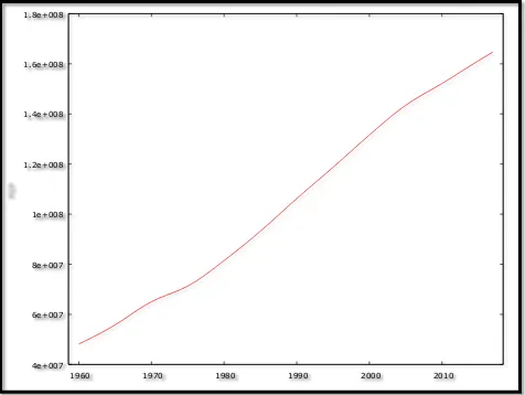
Figure 1 above indicates that the POP variable is not stationary since it is trending upwards over the period 1960 – 2017. This implies that the mean and varience of POP is changing over time.

The Correlogram in Levels

Figure 2

4e+007 6e+007 8e+007 1e+008 1.2e+008 1.4e+008 1.6e+008 1.8e+008

The ADF Test

Table 1: Levels-intercept

Variable ADF Statistic Probability Critical Values Conclusion

POP -1.472889 0.5387 -3.574446 @1% Not stationary

-2.923780 @5% Not stationary -2.599925 @10% Not stationary Table 2: Levels-trend & intercept

Variable ADF Statistic Probability Critical Values Conclusion

POP -4.773851 0.0018 -4.156734 @1% Stationary

-3.504330 @5% Stationary -3.181826 @10% Stationary Table 3: without intercept and trend & intercept

Variable ADF Statistic Probability Critical Values Conclusion

POP -0.834628 0.3492 -2.614029 @1% Not stationary

-1.947816 @5% Not stationary -1.612492 @10% Not stationary

-1 -0.5 0 0.5 1

0 2 4 6 8 10 12

lag ACF for POP

+- 1.96/T^0.5

-1 -0.5 0 0.5 1

0 2 4 6 8 10 12

lag PACF for POP

The Correlogram (at 1st Differences)

Figure 3

Table 4: 1st Difference-intercept

Variable ADF Statistic Probability Critical Values Conclusion

POP -4.363501 0.0011 -3.581152 @1% Stationary

-2.926622 @5% Stationary -2.601424 @10% Stationary Table 5: 1st Difference-trend & intercept

Variable ADF Statistic Probability Critical Values Conclusion

POP -0.271460 0.9894 -4.156734 @1% Not stationary

-3.504330 @5% Not stationary -3.181826 @10% Not stationary Table 6: 1st Difference-without intercept and trend & intercept

-1 -0.5 0 0.5 1

0 2 4 6 8 10 12

lag ACF for d_POP

+- 1.96/T^0.5

-1 -0.5 0 0.5 1

0 2 4 6 8 10 12

lag PACF for d_POP

Variable ADF Statistic Probability Critical Values Conclusion

POP -0.023250 0.6700 -2.614029 @1% Not stationary

-1.947816 @5% Not stationary -1.612492 @10% Not stationary

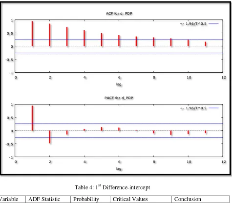
Figures above, i.e. 2 and 3 as well as tables above, i.e. 1 – 6 indicate that the POP series is not stationary at both levels and in first differences.

The Correlogram in (2nd Differences)

Figure 4

Table 7: 2nd Difference-intercept

Variable ADF Statistic Probability Critical Values Conclusion

POP -1.592620 0.4780 -3.584349 @1% Not stationary

-2.928142 @5% Not stationary -2.602225 @10% Not stationary Table 8: 2nd Difference-trend & intercept

Variable ADF Statistic Probability Critical Values Conclusion

-1 -0.5 0 0.5 1

0 2 4 6 8 10 12

lag ACF for d_d_POP

+- 1.96/T^0.5

-1 -0.5 0 0.5 1

0 2 4 6 8 10 12

lag PACF for d_d_POP

POP -3.111448 0.1161 -4.175640 @1% Not stationary -3.513075 @5% Not stationary -3.186854 @10% Not stationary Table 9: 2nd Difference-without intercept and trend & intercept

Variable ADF Statistic Probability Critical Values Conclusion

POP -1.622736 0.0980 -2.617364 @1% Not stationary

-1.948313 @5% Not stationary -1.612229 @10% Stationary

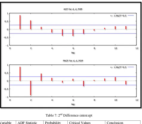
Figure 4 above indicates that most of the autocorrelation coefficients are now closer to zero which is a feature of a stationary series. While tables 7 and 8 show that the POP variable is not yet stationary, table 9 indicates that the POP series is only stationary at 10% level of significance. Non-stationary at 2nd differences points to the fact that the POP series is sharply trending upwards. We could difference the series for the 3rd time but however, for the sake of simplicity, the researcher will however, assume that the POP series is an I (2) variable.

Evaluation of ARIMA models

Table 10

Evaluation of ARIMA models (with a constant)

Model AIC U ME MAE RMSE MAPE

ARIMA (0, 0, 1) 2116.938 10.652 -0.0000376 0 0 20.289

ARIMA (0, 1, 1) 1577.892 0.12569 -2393.4 0.0000209 0.0000241 0.23999

ARIMA (0, 1, 0) 1647.995 0.24004 0 0.0000396 0.0000443 0.44509

ARIMA (0, 2, 0) 1459.113 0.063215 0 79965 0.0000106 0.094804

Evaluation of ARIMA models (without a constant)

ARIMA (0, 2, 1) 1395.057 0.036326 3450.9 45374 60017 0.054789

ARIMA (1, 2, 0) 1379.387 0.031751 294.73 37279 51741 0.044874

ARIMA (2, 2, 0) 1287.544 0.013124 2270.1 17227 22626 0.020926

ARIMA (3, 2, 0) 1271.406 0.011663 1615.9 14984 19493 0.018742

ARIMA (4, 2, 0) 1272.877 0.011614 1539.9 14764 19410 0.018505

ARIMA (4, 2, 1) 1267.442 0.010937 1484.2 14017 18424 0.017414

to select the optimal model in terms of parsimony (AIC) and forecast accuracy (Theil’s U). Therefore, the ARIMA (4, 2, 1) model is chosen.

Residual & Stability Tests

ADF Tests of the Residuals of the ARIMA (4, 2, 1) Model

Table 11: Levels-intercept

Variable ADF Statistic Probability Critical Values Conclusion

εt -2.894582 0.0545 -3.596616 @1% Not stationary

-2.933158 @5% Not stationary -2.604867 @10% Stationary Table 12: Levels-trend & intercept

Variable ADF Statistic Probability Critical Values Conclusion

εt -3.531040 0.0489 -4.192337 @1% Not stationary

-3.520787 @5% Stationary -3.191277 @10% Stationary Table 13: without intercept and trend & intercept

Variable ADF Statistic Probability Critical Values Conclusion

εt -2.965375 0.0040 -2.621185 @1% Stationary

-1.948886 @5% Stationary -1.611932 @10% Stationary

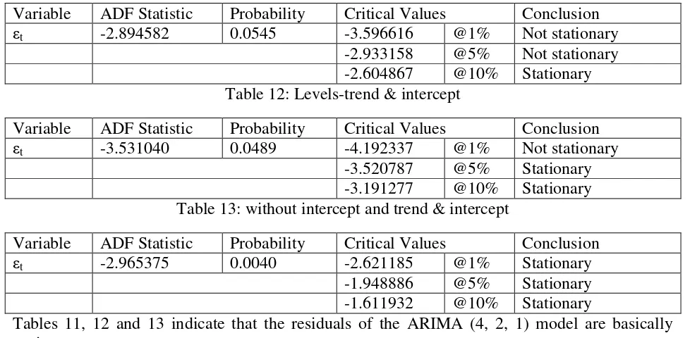
Tables 11, 12 and 13 indicate that the residuals of the ARIMA (4, 2, 1) model are basically stationary.

Stability Test of the ARIMA (4, 2, 1) Model

Figure 5 above indicates that the ARIMA (4, 2, 1) model, is quite stable, since the corresponding inverse roots of the characteristic polynomial lies in the unit circle.

RESULTS & DISCUSSION Descriptive Statistics

Table 14

Description Statistic

Mean 104300000

Median 102290000

Minimum 48200000

Maximum 164670000

Standard deviation 36878000

Skewness 0.099540

Excess kurtosis -1.3647

As shown above in table 14, the mean is positive, i.e. 104300000. The wide gap between the minimum and the maximum is consistent with the reality that the POP series is sharply trending upwards. The skewness is 0.09954 and the most striking characteristic is that it is positive, indicating that the POP series is positively skewed and non-symmetric. Nyoni & Bonga (2017h) reiterate that the rule of thumb for kurtosis is that it should be around 3 for normally distributed variables but in this research, our kurtosis is -1.3647; showing that the POP series is not normally distributed.

-1.5 -1.0 -0.5 0.0 0.5 1.0 1.5

-1.5 -1.0 -0.5 0.0 0.5 1.0 1.5 AR roots

MA roots

Results Presentation1

Table 15

ARIMA (4, 2, 1) Model:

∆2_𝑃𝑂𝑃

𝑡−1= 1.257∆2𝑃𝑂𝑃𝑡−1+ 0.24∆2𝑃𝑂𝑃𝑡−2− 1.279∆2𝑃𝑂𝑃𝑡−3+ 0.609∆2𝑃𝑂𝑃𝑡−4+ 0.875𝜇𝑡−1… . . [2]

P: (0.0000) (0.0366) (0.0000) (0.0000) (0.0000)

S. E: (0.1123) (0.1150) (0.0967) (0.1031) (0.0952)

Variable Coefficient Standard Error z p-value

AR (1) 1.25697 0.112291 11.19 0.0000***

AR (2) 0.240326 0.114954 2.091 0.0366**

AR (3) -1.27882 0.0966986 -13.22 0.0000***

AR (4) 0.609127 0.103109 5.908 0.0000***

MA (1) 0.874603 0.0951558 9.191 0.0000***

Interpretation of Results

Coefficients of the AR (1), AR (3) and AR (4) components are statistically significant at 1% level of significance while the coefficient of the AR (2) component is positive and statistically significant at 5% level of significance. AR terms take the lion’s share in this model, implying that previous population levels are quite relevant in explaining future total annual population of Bangladesh. The MA component (i.e the coefficient 0.874603) is positive and statistically significant at 1% level of significance and this implies that previous disturbances (shocks) to Bangladesh population yield a positive impact on total population in the country.

Forecast Graph

Figure 6

1

Predicted Total Population (for selected years)

Figure 7

1e+008 1.2e+008 1.4e+008 1.6e+008 1.8e+008 2e+008 2.2e+008 2.4e+008 2.6e+008

1990 2000 2010 2020 2030 2040 2050

95 percent interval POP forecast

169829000 173385000

176977000 180517000

184004000 187499000

191035000 194587000

198120000 201631000

205144000 208672000

212208000 215738000

219258000 222778000

2020 2024 2028 2032 2036 2040 2044 2048

Figures 6 (with a forecast range of 32 years, i.e.; 2018 – 2050) and 7, clearly indicate that Bangladesh population is indeed set to continue rising sharply, at least for the next 3 decades; unless and until stern population control measures are put in place. With a 95% confidence interval of 186 890 000 to 258 666 000 and a projected total population of 222 778 000 by 2050, our model is consistent with the population projections by both the Population Reference Bureau (2016) and the UN (2015) which forecasted that Bangladesh’s population will be approximately 202 million by 2050.

POLICY IMPLICATIONS

i. There is need to put in place and enforce family planning policies and practices in Bangladesh.

ii. The government of Bangladesh should promote the smaller family size norm. iii. Sex education must be delivered in order to control fertility in Bangladesh.

CONCLUSION

The ARIMA (4, 2, 1) model is an appropriate and most parsimonious model to forecast the population of Nigeria for the next 3 decades. The model predicts that by 2050, Bangladesh’s population would be approximately, 222 778 000; unless and until more stern population control measures are implemented in Bangladesh. This clearly shows that indeed population growth is a real threat to the future of Bangladesh especially considering the fact that Bangladesh is currently experiencing high levels of unemployment and poverty is widespread. These findings are particulary important for the government of Bangladesh as well as donor organisations, especially when it comes to planning for the future.

REFERENCES

[1] Ahlburg, D. A (1998). Julian Simon and the population growth debate, Population and Development Review, 24: 317 – 327.

[2] Asteriou, D. & Hall, S. G. (2007). Applied Econometrics: a modern approach, Revised Edition, Palgrave MacMillan, New York.

[3] Ayele, A. W & Zewdie, M. A (2017). Modeling and forecasting Ethiopian human population size and its pattern, International Journal of Social Sciences, Arts and Humanities, 4 (3): 71 – 82.

[4] Becker, G., Glaeser, E., & Murphy, K (1999). Population and economic growth,

American Economic Review, 89 (2): 145 – 149.

[5] Beg, A. B. M. R. A & Islam, M. R (2016). Forecasting and modeling population growth of Bangladesh, American Journal of Mathematics and Statistics, 6 (4): 190 – 195.

[7] Du Preez, J. & Witt, S. F. (2003). Univariate and multivariate time series forecasting: An application to tourism demand, International Journal of Forecasting, 19: 435 – 451.

[8] Goh, C. & Law, R. (2002). Modeling and forecasting tourism demand for arrivals with stochastic non-stationary seasonality and intervention, Tourism Management, 23: 499 – 510.

[9] Haque, M., Ahmed, F., Anam, S., & Kabir, R (2012). Future population projection of Bangladesh by growth rate modeling using logistic population model, Annals of Pure and Applied Mathematics, 1 (2): 192 – 202.

[10] Malthus, T (1798). An essay of the principle of population, Pickering, London.

[11] Nyoni, T & Bonga, W. G (2017h). Population growth in Zimbabwe: A Threat to Economic Development? DRJ – Journal of Economics and Finance, 2 (6): 29 – 39.

[12] Nyoni, T (2018l). Modeling Forecasting Naira / USD Exchange Rate in Nigeria: a Box – Jenkins ARIMA approach, University of Munich Library – Munich Personal RePEc Archive (MPRA), Paper No. 88622.

[13] Nyoni, T (2018n). Modeling and Forecasting Inflation in Kenya: Recent Insights from ARIMA and GARCH analysis, Dimorian Review, 5 (6): 16 – 40.

[14] Nyoni, T. (2018i). Box – Jenkins ARIMA Approach to Predicting net FDI inflows in Zimbabwe, Munich University Library – Munich Personal RePEc Archive (MPRA), Paper No. 87737.

[15] Population Reference Bureau (2016). Word Population Data Sheet, PRB, Washington.

[16] Solow, R (1956). Technical change and the aggregate population function, Review of Economics and Statistics, 39: 312 – 320.

[17] Song, H., Witt, S. F. & Jensen, T. C. (2003b). Tourism forecasting: accuracy of alternative econometric models, International Journal of Forecasting, 19: 123 – 141.

[18] Sultana, S., Hasan, M & Andallah, L. S (2015). Age-structured population projection of Bangladesh by using a partial differential model with quadratic polynomial curve fitting, Open Journal of Applied Sciences, 5: 542 – 551.

[19] Tartiyus, E. H., Dauda, T. M., & Peter, A (2015). Impact of population growth on economic growth in Nigeria, IOSR Journal of Humanities and Social Science (IOSR-JHSS), 20 (4): 115 – 123.

[20] Todaro, M & Smith, S (2006). Economic Development, 9th Edition, Vrinda

[21] United Nations (2015). World Population Prospects: The 2015 Revision, Key Findings and Advance Tables, Department of Economic and Social Affairs, Population Division, Working Paper No. ESA/P/WP/241.