Graph based Filtering of Out of Vocabulary Words for Encoder Decoder Models

112

Graph-based Filtering of Out-of-Vocabulary Words

for Encoder-Decoder Models

Satoru Katsumata, Yukio Matsumura∗, Hayahide Yamagishi∗and Mamoru Komachi

Tokyo Metropolitan University

{katsumata-satoru, matsumura-yukio, yamagishi-hayahide}@ed.tmu.ac.jp, [email protected]

Abstract

Encoder-decoder models typically only employ words that are frequently used in the training corpus to reduce the compu-tational costs and exclude noise. How-ever, this vocabulary set may still in-clude words that interfere with learning in encoder-decoder models. This paper pro-poses a method for selecting more suit-able words for learning encoders by uti-lizing not only frequency but also co-occurrence information, which we capture using the HITS algorithm. We apply our proposed method to two tasks: machine translation and grammatical error correc-tion. For Japanese-to-English translation, this method achieves a BLEU score that is 0.56 points more than that of a baseline. Furthermore, it outperforms the baseline method for English grammatical error cor-rection, with anF0.5-measure that is 1.48 points higher.

1 Introduction

Encoder-decoder models (Sutskever et al., 2014) are effective in tasks such as machine translation (Cho et al., 2014; Bahdanau et al., 2015) and grammatical error correction (Yuan and Briscoe, 2016). Vocabulary in encoder-decoder models is generally selected from the training corpus in de-scending order of frequency, and low-frequency words are replaced with an unknown word token <unk>. The so-called out-of-vocabulary (OOV) words are replaced with <unk> to not increase the decoder’s complexity and to reduce noise. However, naive frequency-based OOV replace-ment may lead to loss of information that is nec-essary for modeling context in the encoder.

∗_{Both authors equally contributed to the paper.}

This study hypothesizes that vocabulary con-structed using unigram frequency includes words that interfere with learning in encoder-decoder models. That is, we presume that vocabulary selection that considers co-occurrence informa-tion selects fewer noisy words for learning robust encoders in encoder-decoder models. We apply the hyperlink-induced topic search (HITS) algo-rithm to extract the co-occurrence relations be-tween words. Intuitively, the removal of words that rarely co-occur with others yields better en-coder models than ones that include noisy low-frequency words.

This study examines two tasks, machine transla-tion (MT) and grammatical error correctransla-tion (GEC) to confirm the effect of decreasing noisy words, with a focus on the vocabulary of the encoder side, because the vocabulary on the decoder side is rela-tively limited. In a Japanese-to-English MT exper-iment, our method achieves a BLEU score that is 0.56 points more than that of the frequency-based method. Further, it outperforms the frequency-based method for English GEC, with an F0.5 -measure that is 1.48 points higher.

The main contributions of this study are as fol-lows:

1. The simple but effective preprocessing method we propose for vocabulary selec-tion improves encoder-decoder model perfor-mance.

2. This study is the first to address noise re-duction in the source text of encoder-decoder models.

2 Related Work

et al., 2016) and GEC (Yuan and Briscoe, 2016; Xie et al., 2016; Ji et al., 2017); hence, this study focuses on improving the simple attentional encoder-decoder models that are applied to these tasks.

In the investigation of vocabulary restriction in neural models, Sennrich et al. (2016) applied byte pair encoding to words and created a partial char-acter string set that could express all the words in the training data. They increased the number of words included in the vocabulary to enable the encoder-decoder model to robustly learn contex-tual information. In contrast, we aim to improve neural models by using vocabulary that is appro-priate for a training corpus—not to improve neural models by increasing their vocabulary.

Jean et al. (2015) proposed a method of re-placing and copying an unknown word token with a bilingual dictionary in neural MT. They auto-matically constructed a translation dictionary from a training corpus using a word-alignment model (GIZA++), which finds a corresponding source word for each unknown target word token. They replaced the unknown word token with the corre-sponding word into which the source word was translated by the bilingual dictionary. Yuan and Briscoe (2016) used a similar method for neural GEC. Because our proposed method is performed as preprocessing, it can be used simultaneously with this replace-and-copy method.

Algorithms that rank words using

co-occurrence are employed in many natural

language processing tasks. For example,

TextRank (Mihalcea and Tarau, 2004) uses PageRank (Brin and Page, 1998) for keyword extraction. TextRank constructs a word graph in which nodes represent words, and edges represent co-occurrences between words within a fixed window; TextRank then executes the PageRank algorithm to extract keywords. Although this is an unsupervised method, it achieves nearly the same precision as one state-of-the-art supervised method (Hulth, 2003). Kiso et al. (2011) used HITS (Kleinberg, 1999) to select seeds and create a stop list for bootstrapping in natural language processing. They reported significant improvements over a baseline method using unigram frequency. Their graph-based algorithm was effective at extracting the relevance between words, which cannot be grasped with a simple unigram frequency. In this study, we use HITS

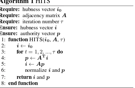
Algorithm 1HITS Require: hubness vectori0

Require: adjacency matrixA

Require: iteration numberτ

Ensure: hubness vectori

Ensure: authority vectorp

1: functionHITS(i0,A,τ)

2: i←i0

3: fort= 1,2, ..., τdo 4: p←AT_i

5: i←Ap

6: normalizeiandp

7: returniandp

8: end function

to retrieve co-occurring words from a training corpus to reduce noise in the source text.

3 Graph-based Filtering of OOV Words

3.1 Hubness and authority scores from HITS

HITS, which is a web page ranking algorithm pro-posed by Kleinberg (1999), computes hubness and authority scores for a web page (node) using the adjacency matrix that represents the web page’s link (edge) transitions. A web page with high au-thority is linked from a page with high hubness scores, and a web page with a high hubness score links to a page with a high authority score. Algo-rithm 1 shows pseudocode for the HITS algoAlgo-rithm. Hubness and authority scores converge by setting the iteration numberτ to a sufficiently large value.

3.2 Vocabulary selection using HITS

In this study, we create an adjacency matrix from a training corpus by considering a word as a node and the co-occurrence between words as an edge. Unlike in web pages, co-occurrence be-tween words is nonbinary; therefore, several co-occurrence measures can be used as edge weights. Section 3.3 describes the co-occurrence measures and the context in which co-occurrence is defined. The HITS algorithm is executed using the adja-cency matrix created in the way described above. As a result, it is possible to obtain a score indi-cating importance of each word while considering contextual information in the training corpus.

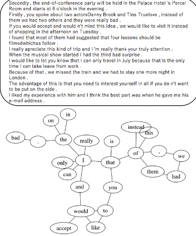
Figure 1 shows a word graph example. A

Figure 1: An example word graph created for ten sentences in the training corpus used for GEC1.

In this study, words with high hubness scores are considered to co-occur with an important word, and low-scoring words are excluded from the vocabulary. Using this method appears to gen-erate a vocabulary that includes words that are more suitable for representing a context vector for encoder models.

3.3 Word graph construction

To acquire co-occurrence relations, we use a com-bination of each word and its peripheral words. Specifically, we combine the target word with sur-rounding words within window widthNand count the occurrences. When defining the context in this way, because the adjacency matrix becomes sym-metric, the same hubness and authority scores can be obtained. Figure 2 shows an example of co-occurrence in whichN is set to two.

We use raw co-occurrence frequency (Freq) and positive pointwise mutual information (PPMI) be-tween words as the (x, y) elementAxy of the

adja-cency matrix. However, naive PPMI reacts sensi-tively to low-frequency words in a training corpus. To account for high-frequency, we weight the PMI by the logarithm of the number of co-occurrences and use PPMI based on this weighted PMI

(Equa-1_{In this study, singleton words and their co-occurrences}

are excluded from the graph.

Figure 2: An example of co-occurrence context.

tion 2).

Af req_xy =|x, y| (1)

Appmi_xy = max(0,pmi(x, y) + log₂|x, y|) (2)

Equation 3 is the PMI of target word x and co-occurrence wordy. M is the number of tokens of the combination, |x,∗|and |∗, y| are the number of token combinations when fixing target wordx

and co-occurrence wordy, respectively.

pmi(x, y) = log₂ M· |x, y|

|x,∗||∗, y| (3)

4 Machine Translation

4.1 Experimental setting

In the first experiment, we conduct a Japanese-to-English translation using the Asian Scientific Paper Excerpt Corpus (ASPEC; Nakazawa et al., 2016). We follow the official split of the train, de-velopment, and test sets. As training data, we use only the first 1.5 million sentences sorted by sen-tence alignment confidence to obtain a Japanese– English parallel corpus (sentences of more than 60 words are excluded). Our training set consists of 1,456,278 sentences, development set consists of 1,790 sentences, and test set consists of 1,812 sentences. The training set has 247,281 Japanese word types and 476,608 English word types.

The co-occurrence window width N is set to two. For combinations that co-occurred only once within the training corpus, we set the value of el-ementAxy of the adjacency matrix to zero. The

iteration numberτ of the HITS algorithm is set to 300. As mentioned in Section 1, we only use the proposed method on the encoder side.

For this study’s neural MT model2, we imple-ment global dot attention (Luong et al., 2015). We train a baseline model that uses vocabulary that is determined by its frequency in the training corpus. Vocabulary size is set to 100K on the encoder side and 50K on the decoder side. Additionally, we

baseline HITS (Freq) HITS (PPMI)

BLEU (50K) 22.24 - 22.40

BLEU (100K) 22.21 22.25 22.77

p-value - 0.35 0.01

Table 1: BLEU scores for Japanese-to-English translation3. The parentheses indicate vocabulary size of the encoder.

COMMON outputs DIFF outputs baseline PPMI baseline PPMI BLEU 22.33 22.98 21.44 21.98

Table 2: BLEU scores of the COMMON and DIFF outputs.

conduct an experiment of varying vocabulary size of the encoder to 50K in the baseline and PPMI to investigate the effect of vocabulary size. Un-less otherwise noted, we conduct an analysis of the model using the vocabulary size of 100K. The number of dimensions for each of the hidden and embedding layers is 512. The mini-batch size is 150. AdaGrad is used as an optimization method with an initial learning rate of 0.01. Dropout is applied with a probability of 0.2.

For this experiment, a bilingual dictionary is prepared for postprocessing unknown words (Jean et al., 2015). When the model outputs an unknown word token, the word with the highest attention score is used as a query to replace the unknown token with the corresponding word from the dic-tionary. If not in the dictionary, we replace the un-known word token with the source word (unk rep). This dictionary is created based on word align-ment obtained using fast align (Dyer et al., 2013) on the training corpus.

We evaluate translation results using BLEU scores (Papineni et al., 2002).

4.2 Results

Table 1 shows the translation accuracy (BLEU scores) and p-value of a significance test (p <

0.05) by bootstrap resampling (Koehn, 2004). The PPMI model improves translation accuracy by 0.56 points in Japanese-to-English translation, which is a significant improvement.

Next, we examine differences in vocabulary by comparing each model with the baseline. Com-pared to the vocabulary of the baseline in 100K setting, Freq and PPMI replace 16,107 and 17,166

3_{BLEU score for postprocessing (unk rep) improves by}

0.46, 0.44, and 0.46 points in the baseline, Freq, and PPMI, respectively.

types, respectively; compared to the vocabulary of the baseline in 50K setting, PPMI replaces 4,791 types.

4.3 Analysis

According to Table 1, the performance of Freq is almost the same as that of the baseline. When examining the differences in selected words in vocabulary between PPMI and Freq, we find that PPMI selects more low-frequency words in the training corpus compared to Freq, because PPMI deals with not only frequency but also co-occurrence.

The effect of unk rep is almost the same in the baseline as in the proposed method, which indi-cates that the proposed method can be combined with other schemes as a preprocessing step.

As a comparison of the vocabulary size 50K and 100K, the BLEU score of 100K is higher than that of 50K in PPMI. Moreover, the BLEU scores are almost the same in the baseline. We suppose that the larger the vocabulary size of encoder, the more noisy words the baseline includes, while the PPMI filters these words. That is why the pro-posed method works well in the case where the vocabulary size is large.

To examine the effect of changing the vocab-ulary on the source side, the test set is divided into two subsets: COMMON and DIFF. The for-mer (1,484 sentences) consists of only the com-mon vocabulary between the baseline and PPMI, whereas the latter (328 sentences) includes at least one word excluded from the common vocabulary. Table 2 shows the translation accuracy of the COMMON and DIFF outputs. Translation perfor-mance of both corpora is improved.

In order to observe how PPMI improves COM-MON outputs, we measure the similarity of the baseline and PPMI output sentences by count-ing the exact same sentences. In the COMMON outputs, 72 sentence pairs (4.85%) are the same, whereas 9 sentence pairs are the same in the DIFF outputs (2.74%). Surprisingly, even though it uses the same vocabulary, PPMI often outputs different but fluent sentences.

src 有用 物質 の 分離 ・ 抽出,反応 性 向上,新 材料 創製,廃棄 物 処理,分析 等 の 分野 が ある 。 baseline there are fields such as separation , extraction , extraction , improvement of new material creation , waste treatment ,

analysis , etc .

Freq there are separation and extraction of useful substances , the improvement of reactivity , new material creation , waste treatment and analysis .

PPMI there are the fields such as separation and extraction of useful materials , the reaction improvement , new material creation , waste treatment , analysis , etc ...

ref the application fields are separation and extraction of useful substances , reactivity improvement , creation of new products , waste treatment , and chemical analysis .

Table 3: An example of Japanese-to-English translation on a source sentence from COMMON.

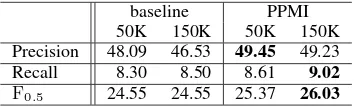
baseline PPMI 50K 150K 50K 150K Precision 48.09 46.53 49.45 49.23 Recall 8.30 8.50 8.61 9.02

F0.5 24.55 24.55 25.37 26.03

Table 4:F0.5 results on the CoNLL-14 test set4.

COMMON outputs DIFF outputs baseline PPMI baseline PPMI P 48.26 60.07 9.40 17.32 R 0.01 0.01 0.01 0.02

F0.5 0.04 0.04 0.04 0.08

Table 5:F0.5of COMMON and DIFF outputs.

5 Grammatical Error Correction

5.1 Experimental setting

The second experiment addresses GEC. We com-bine the FCE public dataset (Yannakoudakis et al., 2011), NUCLE corpus (Dahlmeier et al., 2013), and English learner corpus from the Lang-8 learner corpus (Mizumoto et al., 2011) and re-move sentences longer than 100 words to create a training corpus. From the Lang-8 learner pus, we use only the pairs of erroneous and cor-rected sentences. We use 1,452,584 sentences as a training set (502,908 types on the encoder side and 639,574 types on the decoder side). We evalu-ate the models’ performances on the standard sets from the CoNLL-14 shared task (Ng et al., 2014) using CoNLL-13 data as a development set (1,381 sentences) and CoNLL-14 data as a test set (1,312 sentences)4. We employ F0.5 as an evaluation measure for the CoNLL-14 shared task.

We use the same model as in Section 4.1 as a neural model for GEC. The models’ parameter set-tings are similar to the MT experiment, except for the vocabulary and batch sizes. In this experiment, we set the vocabulary size on the encoder and de-coder sides to 150K and 50K, respectively.

Ad-4_{We do not consider alternative answers suggested by the}

participating teams.

src Genetic refers the chance of inheriting a dis-order or disease .

baseline Genetic refers the chance of inheriting a dis-order or disease .

PPMI Genetic referstothe chance of inheriting a disorder or disease .

gold Geneticriskreferstothe chance of inherit-ing a disorder or disease .

Table 6: An example of GEC using a source sen-tence from COMMON.

ditionally, we conduct the experiment of changing vocabulary size of the encoder to 50K to investi-gate the effect of the vocabulary size. Unless oth-erwise noted, we conduct an analysis of the model using the vocabulary size of 150K. The mini-batch size is 100.

5.2 Result

Table 4 shows the performance of the baseline and proposed method. The PPMI model improves pre-cision and recall; it achieves aF0.5-measure 1.48 points higher than the baseline method.

In setting the vocabulary size of encoder to 150K, PPMI replaces 37,185 types from the base-line; in the 50K setting, PPMI replaces 10,203 types.

5.3 Analysis

TheF0.5of the baseline is almost the same while the PPMI model improves the score in the case where the vocabulary size increases. Similar to MT, we suppose that the PPMI filters noisy words. As in Section 4.3, we perform a follow-up ex-periment using two data subsets: COMMON and DIFF, which contain 1,072 and 240 sentences, re-spectively.

Table 5 shows the accuracy of the error correc-tion of the COMMON and DIFF outputs. Preci-sion increases by 11.81 points, whereas recall re-mains the same for the COMMON outputs.

dif-MT GEC baseline PPMI baseline PPMI tokens 52,700 27,364 126,884 70,003 Ave. tokens 3.07 1.59 3.36 1.85

Table 7: Number of words included only in either the baseline or PPMI vocabulary.

ferences in the training environment. Unlike MT, we can copy OOV in the target sentence from the source sentence without loss of fluency; therefore, our model has little effect on recall, whereas its precision improves because of noise reduction.

Table 6 shows an example of GEC. The pro-posed method’s output improves when the source sentence is expressed using common vocabulary.

6 Discussion

We described that the proposed method has a pos-itive effect on learning the encoder. However, we have a question; what affects the performance? We conduct an analysis of this question in this sec-tion.

First, we count the occurrence of the words in-cluded only in the baseline or PPMI in the training corpus. We also show the number of the tokens per types (“Ave. tokens”) included only in either the baseline or PPMI vocabulary.

The result is shown in Table 7. We find that the proposed method uses low-frequency words in-stead of high-frequency words in the training cor-pus. This result suggests that the proposed method works well despite the fact that the encoder of the proposed method encounters more <unk> than the baseline. This is because the proposed method excludes words that may interfere with the learn-ing of encoder-decoder models.

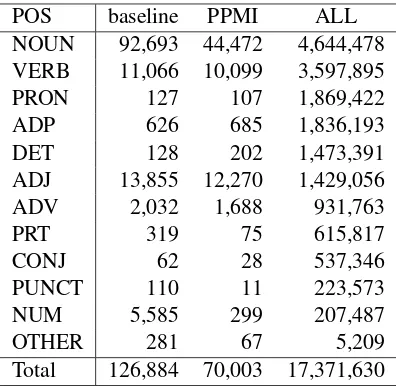
Second, we conduct an analysis of the POS of the words in GEC to find why increasing OOV improves the learning of encoder-decoder models. Specifically, we apply POS tagging to the training corpus and calculate the occurrence of the POS of the words only included in the baseline or PPMI. We use NLTK as a POS tagger.

Table 8 shows the result. It is observed that NOUN is the most affected POS by the proposed method and becomes often represented by<unk>. NOUN words in the vocabulary of the baseline contain some non-English words, such as Japanese or Korean. These words should be treated as OOV but the baseline fails to exclude them using only the frequency. According to Table 8, NUM is also

POS baseline PPMI ALL

NOUN 92,693 44,472 4,644,478

VERB 11,066 10,099 3,597,895

PRON 127 107 1,869,422

ADP 626 685 1,836,193

DET 128 202 1,473,391

ADJ 13,855 12,270 1,429,056

ADV 2,032 1,688 931,763

PRT 319 75 615,817

CONJ 62 28 537,346

PUNCT 110 11 223,573

NUM 5,585 299 207,487

OTHER 281 67 5,209

Total 126,884 70,003 17,371,630

Table 8: Number of the POS of words only in-cluded in the baseline or PPMI.

affected by the proposed method. NUM words of the baseline include a simple numeral such as “119”, in addition to incorrectly segmented nu-merals such as “514&objID”. This word appears 25 times in the training corpus owing to the noisy nature of Lang-8. We suppose that the proposed method excludes these noisy words and has a pos-itive effect on training.

7 Conclusion

In this paper, we proposed an OOV filtering method, which considers word co-occurrence in-formation for encoder-decoder models. Unlike conventional OOV handling, this graph-based method selects the words that are more suitable for learning encoder models by considering con-textual information. This method is effective for not only machine translation but also grammatical error correction.

This study employed a symmetric matrix (sim-ilar to skip-gram with negative sampling) to ex-press relationships between words. In future re-search, we will develop this method by using vocabulary obtained by designing an asymmetric matrix to incorporate syntactic relations.

Acknowledgments

References

Dzmitry Bahdanau, Kyunghyun Cho, and Yoshua Ben-gio. 2015. Neural machine translation by jointly learning to align and translate. InProc. of ICLR.

Sergey Brin and Lawrence Page. 1998. The anatomy of a large-scale hypertextual web search engine.Comput. Netw. ISDN Syst.30(1-7):107–117. https://doi.org/10.1016/S0169-7552(98)00110-X.

Kyunghyun Cho, Bart van Merrienboer, Caglar Gulcehre, Dzmitry Bahdanau, Fethi Bougares, Holger Schwenk, and Yoshua Bengio. 2014. Learning phrase representations using RNN encoder–decoder for statistical machine trans-lation. In Proc. of EMNLP. pages 1724–1734. http://www.aclweb.org/anthology/D14-1179.

Daniel Dahlmeier, Hwee Tou Ng, and Siew Mei Wu. 2013. Building a large annotated cor-pus of learner English: The NUS corpus of learner English. In Proc. of BEA. pages 22–31. http://www.aclweb.org/anthology/W13-1703.

Chris Dyer, Victor Chahuneau, and Noah A. Smith. 2013. A simple, fast, and effec-tive reparameterization of IBM model 2.

In Proc. of NAACL-HLT. pages 644–648.

http://www.aclweb.org/anthology/N13-1073.

Anette Hulth. 2003. Improved automatic key-word extraction given more linguistic knowl-edge. In Proc. of EMNLP. pages 216–223. http://www.aclweb.org/anthology/W03-1028.

S´ebastien Jean, Orhan Firat, Kyunghyun Cho, Roland Memisevic, and Yoshua Bengio. 2015. Montreal neural machine translation systems for WMT15. In Proc. of WMT. pages 134–140. http://aclweb.org/anthology/W15-3014.

Jianshu Ji, Qinlong Wang, Kristina Toutanova, Yongen Gong, Steven Truong, and Jianfeng Gao. 2017. A nested attention neural hybrid model for grammat-ical error correction. In Proc. of ACL. pages 753– 762. http://aclweb.org/anthology/P17-1070.

Tetsuo Kiso, Masashi Shimbo, Mamoru Komachi, and Yuji Matsumoto. 2011. HITS-based seed selection and stop list construction for boot-strapping. In Proc. of ACL. pages 30–36. http://www.aclweb.org/anthology/P11-2006.

Jon M. Kleinberg. 1999. Authoritative sources in a hyperlinked environment. J. ACM 46(5):604–632. https://doi.org/10.1145/324133.324140.

Philipp Koehn. 2004. Statistical signifi-cance tests for machine translation evalua-tion. In Proc. of EMNLP. pages 388–395. http://www.aclweb.org/anthology/W04-3250.

Thang Luong, Hieu Pham, and Christopher D. Manning. 2015. Effective approaches to attention-based neural machine translation.

In Proc. of EMNLP. pages 1412–1421.

http://aclweb.org/anthology/D15-1166.

Rada Mihalcea and Paul Tarau. 2004. TextRank: Bringing order into texts. InProc. of EMNLP. pages 404–411. http://www.aclweb.org/anthology/W04-3252.

Tomoya Mizumoto, Mamoru Komachi, Masaaki Na-gata, and Yuji Matsumoto. 2011. Mining re-vision log of language learning sns for auto-mated Japanese error correction of second language learners. In Proc. of IJCNLP. pages 147–155. http://www.aclweb.org/anthology/I11-1017.

Toshiaki Nakazawa, Manabu Yaguchi, Kiyotaka Uchi-moto, Masao Utiyama, Eiichiro Sumita, Sadao Kurohashi, and Hitoshi Isahara. 2016. ASPEC: Asian scientific paper excerpt corpus. In Proc. of LREC. pages 2204–2208.

Hwee Tou Ng, Siew Mei Wu, Ted Briscoe, Christian Hadiwinoto, Raymond Hendy Susanto, and Christo-pher Bryant. 2014. The CoNLL-2014 shared task on grammatical error correction. InProc. of CoNLL Shared Task. pages 1–14.

Kishore Papineni, Salim Roukos, Todd Ward, and Wei-Jing Zhu. 2002. BLEU: a method for automatic evaluation of machine trans-lation. In Proc. of ACL. pages 311–318. http://www.aclweb.org/anthology/P02-1040.

Hinrich Sch¨utze. 1998. Automatic word sense discrim-ination. Computational Linguistics 24(1):97–123. http://dl.acm.org/citation.cfm?id=972719.972724.

Rico Sennrich, Barry Haddow, and Alexandra Birch. 2016. Neural machine translation of rare words with subword units. InProc. of ACL. pages 1715–1725. http://www.aclweb.org/anthology/P16-1162.

Ilya Sutskever, Oriol Vinyals, and Quoc V Le. 2014. Sequence to sequence learning with neural net-works. InProc. of NIPS. pages 3104–3112.

Yonghui Wu, Mike Schuster, Zhifeng Chen, Quoc V Le, Mohammad Norouzi, Wolfgang Macherey, Maxim Krikun, Yuan Cao, Qin Gao, Klaus Macherey, et al. 2016. Google’s neural ma-chine translation system: Bridging the gap between human and machine translation. arXiv preprint arXiv:1609.08144.

Ziang Xie, Anand Avati, Naveen Arivazhagan, Dan Ju-rafsky, and Andrew Y Ng. 2016. Neural language correction with character-based attention. arXiv preprint arXiv:1603.09727.