Munich Personal RePEc Archive
Bangladesh’s Trade Partners and the
J-Curve: An Asymmetry Analysis
BAHMANI-OSKOOEE, Mohsen and Rahman, Mir Obaidur
and Kashem, Muhammad
University of Wisconsin-Milwaukee, Department of Economics,
United International University, Dhaka, Bangladesh, Department of
Economics, Bangladesh Bank, Dhaka, Bangladesh
6 August 2017
Online at
https://mpra.ub.uni-muenchen.de/81208/
1
Bangladesh’s Trade
Partners and the J-Curve: An Asymmetry Analysis
Mohsen Bahmani-Oskooee
The Center for Research on International Economics Department of Economics
The University of Wisconsinin-Milwaukee, Milwaukee, WI bahmani@uwm.edu
Mir Obaidur Rahman Department of Economics School of Business and Economics
United International University, Dhaka, Bangladesh obaidur@eco.uiu.ac.bd
Mohammad Abul Kashem Joint Director Bangladesh Bank kashem24bb@gmail.com
ABSTRACT
Separating currency appreciations from depreciations and using nonlinear models in recent literature have improved discovering significant link between the trade balance and the exchange rate. We add to this growing literature by considering the experience of Bangladesh with 11 trading partners. When a linear model was used, support for the J-curve effect was present only with one small partner. However, when a nonlinear model was used, support increased to three countries including the largest partner, the U.S. which accounts for more than 12% of Bangladesh’s trade. Furthermore, the nonlinear models supported short-run asymmetry adjustment as well as short-run asymmetry effects of exchange rate changes in most cases. However, long-run asymmetric effects were limited to a few.
Keywords:Bangladesh, Taka, J-curve, Asymmetry Analysis, 11 Partners
2
1. Introduction
Methodological advances in economics always encourage researchers to revisit old theories
and the link between the trade balance and the exchange rate is no exception. While standard OLS
method used to be applied between the trade balance and its determinants, including the exchange
rate, introduction of the error-correction modeling approach and co-integration technique opened
another path to distinguish the short-run from the long-run effects. Indeed, it is argued in the
literature that a devaluation or depreciation could worsen the trade balance in the short run but improve it in the long run, hence the “J-curve” phenomenon. Two review articles by
Bahmani-Oskooee and Ratha (2004) and Bahmani-Bahmani-Oskooee and Hegerty (2010) reveal that every country
has its own literature and our country of concern, Bangladesh, must be no exception.1
Studies related to the experience of Bangladesh with the J-curve effect are rare, perhaps due to
lack of data. The two studies that have assessed the impact of currency depreciation on the trade
balance of Bangladesh, have both found support for favorable effects of depreciation in the long
run, but mixed results in the short run. While Khatoon and Rahman (2009) used annual data over
1972-2006 periods to arrive at their estimates, Aziz (2012) used annual data over the period
1976-2009. Clearly, thirty some observations do not leave us with enough degrees of freedom to make
a reliable inference. Furthermore, both studies suffer from aggregation bias in that they have used
aggregate trade flows of Bangladesh with the rest of the world. The implication is that a
devaluation or depreciation may improve Bangladesh’s trade balance with some but not with all
trading partners. Thus, in order to identify trading partners against whom a depreciation of Taka
will improve Bangladesh’s trade balance, we disaggregate Bangladesh’s trade flows by its major
1 Note that while Magee (1973) and Junz and Rhomberg (1973) introduced the J-curve concept theoretically,
3 partners and try to test the J-curve effect at bilateral level. However, in order to learn about
importance of each partner in Bangladesh’s trade, we plot their trade share in Figure 1 below:2
Figure 1: Trade Shares of Each Partner
As can be seen, the 11 partners for whom continuous data were available engage in almost 65% of
trade with Bangladesh. The U.S. happens to be the largest partner.
Reducing or dismembering aggregation bias by estimating the trade balance at bilateral
level was originally raised against the aggregate literature by Rose and Yellen (1989). However,
recently Rose and Yellen (1989) approach was criticized by Bahmani-Oskooee and Fariditavana
(2016) for assuming the effects of bilateral exchange rate changes on the bilateral trade balance to
be symmetric. After arguing for possibility of asymmetric effects, they provide empirical evidence
2Each trade share is defined as sum of Bangladesh’s exports to and imports from each partner as a percent of sum of
4 supporting asymmetric effects of exchange rate changes in the short-run and long-run.
Asymmetries arise, as they argue, because of asymmetry pass-through of exchange rate changes
to import and export prices and because of change in traders’ expectations and behavior. Therefore,
our goal in this paper is to assess the asymmetric effects of changes in the value of Taka on the
trade balance of Bangladesh with each of her 11 partners depicted in figure 1. For that purpose, in
Section II we introduce the models and methods. Empirical results are presented in Section III
with a summary in Section IV. Data definition and sources are cited in an Appendix.
2.
The Models and MethodsSince Bahmani-Oskooee and Fariditavana’s (2016) approach of asymmetry analysis is the
latest advance in the trade balance literature, we begin with their specification of the trade balance
model first as outlined by (1):
where TBiis Bangladesh’s trade balance with trading partner i. Since the model is specified in
logarithmic form, the trade balance is defined as the ratio of Bangladesh’s imports from partner i
over her exports to partner i. The main reason for using the ratio of imports over exports and not
the other way around is the definition of the real bilateral exchange rate (REXi). As the Appendix
reveals, it is defined in a manner that a decline signifies Taka depreciation. Thus, if a real
depreciation of Taka against partner i’s currency is to improve Bangladesh’s trade balance with
partner i, an estimate of d should be positive. In (1), YBDdenotes Bangladesh’s real income and
since an increase in it is expected to boost Bangladesh’s imports, an estimate of b is expected to )
1 (
, ,
,
,t BD t it it t
i a bLnY cLnY dLnREX
5 be positive. Finally, Yi denotes partner i’s income and since an increase in it is expected to boost
Bangladesh’s exports to that partner, and estimate of d is expected to be negative.3
The next step in our model building approach is to introduce the short-run dynamic
adjustment process into (1) by turning it to an error-correction model as specified by (2):
) 2 ( 1 , 4 1 , 3 1 , 2 1 , 1 , 0 , 0 , 0 , 1 , t t i t i t BD t i j t i n j j t j t i n j j t j t BD n j j t j t i n j j t t i LnREX LnY LnY LnTB LnREX LnY LnY LnTB LnTB
Specification (2) is an error-correction model where the short-run effects of each variable on the
trade balance is inferred by the estimate of coefficients attached to the first-differenced variables
and the long-run effects are judged by the estimate of λ2–λ4 normalized on λ1. However, for these
normalized estimates to be meaningful, we must establish co-integration. Since the approach is
due to Pesaran et al. (2001), they recommend applying the F test for which they tabulate new
critical values. Since the critical values do account for degrees of integration of variables, there is
no need for pre-unit root testing and variables could be combination of I(0) and I(1).
The main assumption in (2) is that changes in any of the variables have symmetric effects
on the trade balance. Concentrating on the exchange rate, the symmetry assumption implies that
Taka depreciation has the same effect on the trade balance as Taka appreciation in size but not in
sign. However, Bahmani-Oskooee and Fariditavana (2016) argued to the contrary and for
3 Of course, income elasticities could take opposite signs if increase in income is due to an increase in production of
6 asymmetric effects since traders’ reaction could be different to appreciations as compared to
depreciations. They then followed Shin et al.’s (2014) approach and changed (2) to a new
specification that could be used to assess the asymmetric effects of exchange rate changes as
follows:
As can be seen, in moving from (2) to (3), the LnREX variable has been replaced by two new
variables, POS and NEG where POS is defined as partial sum of positive changes in LnREX and
reflects only currency appreciation. By the same token, the NEG variable is defined as partial sum
of negative changes in LnREX and reflects only Taka depreciations.4 Since constructing the two
partial sum variables introduce nonlinear adjustment of exchange rate changes into our
error-correction model, specifications such as (3) are known as nonlinear ARDL models, whereas the
ones similar to (2) that assumes symmetric effects are known as the linear ARDL models.
Shin et al. (2014) have demonstrated that once (3) is estimated by the OLS, it could be
used to assess asymmetric co-integration and several additional asymmetric effects of exchange
rate changes on the trade balance. First, the same F test is used to establish joint significance of
4Note that in order to generate the two partial sum variables; we first form ΔLnREXt which includes positive and
negative changes. Then POSt at any given period t is defined as cumulative sum all observations in ΔLnREXt where negative values are replaced with zeroes. The NEGt variable is defined the same way where positive values of
ΔLnREXt are replaced with zeroes. For exact formulation of these two partial sums see Bahmani-Oskooee and
7 lagged level variables as a sign of asymmetry co-integration. Here, Shin et al. (2014, p. 291) even
recommend treating the POS and NEG variables as a single variable so that the critical values of
the F test stay at the same conservative level when we move from (2) to (3), though (3) has one
more variable. This is mostly due to dependency between the two partial sum variables. Second,
the same alternative test that is used for co-integration in the linear model (2) is also used in the
nonlinear model (3). In this alternative test that is known as ECMt-1 test, normalized long-run
estimates from (3) and a long-run model (1) in which the LnREX is replaced by POS and NEG
variables are used to generate the error term, denoted as ECM. After replacing the linear
combination of lagged level variables in (3) by ECMt-1, the new specification is estimated at the
same optimum lags as before. A significantly negative coefficient attached for ECMt-1 will be an
alternative way of supporting co-integration. However, just like the F test, the t-test that is used to
judge significance of this estimate has a new distribution for which Pesaran et al. (2001, P. 303)
tabulate new upper and lower bound critical values.
Second, if at each lag j, estimate of e’j is different than estimate of f’j, that will be an
indication of short-run asymmetric effects of exchange rate changes on the trade balance.
However, if
'
ˆ'ˆj fj
e , this will be an indication of short-run cumulative or impact asymmetry.
The Wald test will be used to test this inequality. Third, if optimum number of lags on ΔPOS is
different than the number of lags on ΔNEG, that will be a sign of short-run “adjustment
asymmetry”. Finally, if we establish that
0 4
0 3
ˆ ˆ ˆ ˆ
, i.e., normalized estimate attached to the
8 which will be an indication of long-run asymmetric effects. Again, the Wald test will be used to
establish this inequality. Both linear and nonlinear models are estimated in the next section.5
3.
Empirical Results
In this section we estimate both models between Bangladesh and each of her 11 major partners
displayed in figure 1. These 11 partners, i.e. China, United States, India, Germany, Singapore,
United Kingdom, Canada, France, Japan, Korea and Malaysia engage in almost 65% of total
Bangladesh’s trade. Quarterly data over the period 1985I-2015IV are used to carry out the
empirical exercise. Furthermore, a maximum of four lags are imposed on each first-differenced
variable and Akaike’s Information Criterion is used to select an optimum model. Since there are
different critical values for different estimate (coefficient or diagnostic), they are collected in the
notes to Table 1 and are used to indicate significant levels. Any significant estimate at the 10%
level is indicated by * and those at 5% level by **. Note also that an estimate of the linear model
is headed by L-ARDL and those of the nonlinear model by NL-ARDL.
Table 1 goes about here
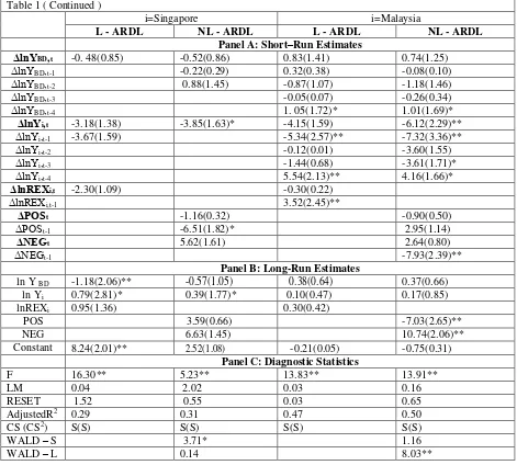
From the short-run coefficient estimates of the linear ARDL models that are reported in
Panel A, we gather that the real exchange rate carries at least one significant coefficient in the
models where Germany, China, and Malaysia are trading partners. However, when we consider
the results from nonlinear models, it appears that either ΔPOS or ΔNEG carry at least one
significant coefficient in the cases of USA, Canada, France, Germany, India, Japan, Korea,
Singapore and Malaysia. Clearly, the increase from three partners in the linear model to nine in
5 For more on some other application of these methods see Gogas and Pragidis (2015), Durmaz (2015), Baghestani
9 the nonlinear model which includes the largest partner, the US, must be attributed to nonlinear
adjustment of the real bilateral exchange rate. This by itself supports application of nonlinear
models.
In addition to providing relatively more support for the short-run effects of exchange rate
changes on Bangladesh’s trade balances, the nonlinear models also support short-run adjustment
asymmetry in the models that belong to the U.S., U.K., France, Germany, China, India, Japan,
Korea, Singapore, and Malaysia since in these cases ΔPOS takes a different lag order than ΔNEG.
Furthermore, the size of short-run coefficient estimates attached to ΔPOS and ΔNEG are different
at almost all the same lags. This indeed, supports short-run asymmetric effects of exchange rate
changes on Bangladesh’s bilateral trade balances. However, the sum of coefficients attached to
ΔPOS are significantly different than the sum attached to ΔNEG only in the results for the U.S.,
Canada, Germany, and Singapore since in these cases the Wald statistics reported as the Wald-S
in Panel C are significant. Do these short-run asymmetric effects translate into the long run?
The long-run coefficient estimates are reported in Panel B. Estimates from the L-ARDL
models reveal that the real bilateral exchange rate carries a significant normalized coefficient only
in the results with Canada and Korea. In the case of Canada, while Taka depreciation will improve Bangladesh’s trade balance with Canada, in the results with Korea, it will hurt. This could be due
to either an inelastic Korean demand for Bangladesh’s goods or an inelastic demand by Bangladesh
for Korean goods. However, when we shift to NL-ARDL models, we gather that either POS or
NEG carry a significant normalized long-run coefficient in the models that belong to the U.S.,
Canada, UK, and Malaysia. Furthermore, the long-run effects are asymmetric in the cases of the
U.S., France, and Malaysia since the Wald test reported as the Wald-L in Panel C are significant
10 As for the J-curve effect, not much support is found by either model. The linear model
supports Rose and Yellen (1989) definition only in the case of Canada since short-run insignificant
results are combined with significant and positive long-run estimate for the exchange rate variable.
The nonlinear model supports Bahmani-Oskooee and Fariditavana’s (2016) definition in the cases
of the U.S., Canada, and Malaysia. In the nonlinear models that belong to these three partners,
insignificant short-run results are combined with significantly positive coefficient obtained either
for POS or NEG variable. Again, separating appreciations from depreciations and introducing
nonlinear adjustment of the real bilateral exchange rate is the reason for the increase from one
partner to three in which asymmetry J-curve is supported. Clearly, the results are partner-specific.
For example, consider the models with the largest partner, the U.S. If we were to rely upon the
nonlinear model only, we would have concluded that the real rate has no long-run effects on the
trade balance of Bangladesh with the U.S. However, the nonlinear model predicts that while Taka
depreciation will have no effect, Taka appreciation will hurt Bangladesh’s trade balance with the
U.S. On the other hand, the linear Bangladesh-Canadian model predicts that Taka depreciation
against Canadian dollar will improve the bilateral trade balance and Taka appreciation will hurt it.
However, the nonlinear model reveals that there is no room for Taka depreciation to be effective
but Taka appreciation will hurt the bilateral trade balance.
All long-run estimates reviewed above as well as significant long-run income elasticities
are valid since co-integration among variables of both models are supported by the F test. As can
be seen, all F statistics reported in Panel C are significant. We have also reported a few additional
diagnostic statistics in Panel C. To test for autocorrelation, we have reported the Lagrange
Multiplier statistics as LM. Since it is insignificant in all models, residuals are autocorrelation free
11 RESET test. It is significant only in the bilateral models with Germany, leaving the remaining
optimum models as correctly specified. To establish stability of short-run and long-run coefficient
estimates we have applied the well-known CUSUM and CUSUMSQ and indicated these tests by
CS and CS2 in Panel C. Stable estimates are identified by “S” and unstable ones by “UNS”. As
can be seen, most estimates are stable. Lastly, the size of adjusted R2 is reported to judge the
goodness of fit.
4.
Summary and Conclusion
The link between the trade balance and the real exchange rate has now entered into a new path
due to introduction of possibility of asymmetric response of the trade balance to exchange rate
changes. The evidence in the literature is abundant enough to expect asymmetric response. Since
asymmetry analysis necessitates application of nonlinear models, nonlinear adjustment of the real
exchange rate is said to be the main contributing factor. In this paper we add to the growing
literature by considering experience of Bangladesh, a country that has been ignored by most
previous studies, perhaps being small or due to lack of continuous time-series data.
Using quarterly data over the period 1985Q1-2015Q4 we consider the bilateral trade balances
of Bangladesh with each of her 11 major trading partners. Together, these 11 partners engage in
65% of Bangladesh trade and the list ranked in terms of declining order include the U.S. (12.28%),
India (7.7%), Canada (7.32%), Japan (5.87%), Germany (5.62%), Singapore (5.06%), U.K.
(4.78%), Korea (2.89%); France (2.61%), Canada (2.1%), and Malaysia (1.64%).
When we applied the linear ARDL approach of Pesaran et al. (2001) to 11 trade balance
models, we were able to find support for the J-curve effect, i.e., negative or insignificant short-run
12 the model with Canada. However, when we separated currency appreciations from depreciations
and relied upon Shin et al.’s (2014) nonlinear ARDL approach, support for the J-curve increased
to three countries, i.e., U.S., Canada, and Malaysia. Estimates of the nonlinear models yielded
additional information with regards to asymmetric effects of exchange rate changes. With most
partners, short-run effects were asymmetric but long-run asymmetric effects were limited to a few
partners only. Future research should concentrate on Bangladesh trade with each major partner but
disaggregate trade flows by commodity in order to determine how each industry responds to
13
A
ppendix
Data Definition and Sources
Quarterly data over the period 1985Q1-2015Q4 are used to carry out the empirical exercise for all the countries. The following sources were used to collect the required data:
a. International Financial Statistics, IMF. b. Bangladesh Bureau of Statistics.
c. Direction of Trade Statistics (DOTS), IMF d. European Central Bank webpage,
https//wwwecb.europa.eu/press/pr/date/1998/html/pr98123-2.en.html
Variables:
TBi = Bangladesh’s trade balance with partner i. This is defined as Bangladesh imports from the
partner i over her exports to partner i. (Mi/Xi ). Data come from source c.
Yi = Real GDP of partner i (base year 2010). The data come from source a.
YBD= Real GDP of Bangladesh. Quarterly real GDP data are not available for Bangladesh, they were generated following an interpolation method by Bahmani-Oskooee (1986, p. 23).
REX = Real bilateral exchange rate defined as (PBD. NEX)/Pi where NEX is the nominal bilateral exchange rate defined as the number of units of partner i’s currency per unit of Taka. Thus, a decline in REX reflects a real depreciation of the Bangladeshi Taka. Consumer Price Index (CPI) of Bangladesh is from Source b and for other countries the source is a. The base year price level for all countries is 2010.
All nominal bilateral exchange rates between Taka and country i’s currency were generated using the rates against the U.S. dollar. All data come from source a.
14
REFERENCES
Aftab, M., R. Ahmad, I. Ismail and M. Ahmed (2017) “Exchange Rate Volatility and
Malaysian-Thai Bilateral Industry Trade Flows”, Journal of Economic Studies, Vol.44, pp.99-114.
Al-Shayeb, A. and A. Hatemi-J. (2016) "Trade Openness and Economic Development in the UAE: An Asymmetric Approach", Journal of Economic Studies, Vol. 43, pp.587-597.
Arize, A. C., J. Malindretos, and E.U. Igwe, (2017), “Do Exchange Rate Changes Improve the Trade Balance: An Asymmetric Nonlinear Co-integration Approach”, International Review of
Economics and Finance, Vol. 49, pp. 313-326.
Aziz, N. (2012), “Does a Real Devaluation Improve the Balance of Trade? Empirics from Bangladesh Economy”, The Journal of Developing Areas, Vol. 46, 19-41.
Baghestani, H. and S. Kherfi, (2015) "An Error-correction Modeling of US Consumer Spending: Are There Asymmetries?", Journal of Economic Studies, Vol. 42, pp.1078-1094.
Bahmani-Oskooee, M. (1985) “Devaluation and the J-Curve: Some Evidence from LDCs”,The
Review of Economics and Statistics, Vol. 67, 500-504.
Bahmani-Oskooee, M. (1986), "Determinants of International Trade Flows: Case of Developing
Countries," Journal of Development Economics, Vol. 20, 107-123.
Bahmani-Oskooee, M. and Fariditavana, H. (2016) “Nonlinear ARDL Approach and the J Curve Phenomenon,” Open Economies Review, 27, 51-70.
Bahmani-Oskooee, M. and Hegerty, S.W. (2010) “The J- and S-Curves: A Survey of the Recent Literature”, Journal of Economic Studies 37(6), 580-596.
Bahmani-Oskooee, M and Ratha (2004), The J- Curve: A literature review, Applied Economics,
36(13), 1377-1398.
Durmaz, N. (2015) “Industry level J-curve in Turkey”, Journal of Economic Studies, Vol.42, No.4, pp.689-706.
Gogas, P. and I. Pragidis, (2015) "Are There Asymmetries in Fiscal Policy hocks?", Journal
of Economic Studies, Vol.42, pp.303-321.
Gregoriou, A. (2017) "Modelling non-linear behaviour of block price deviations when trades are executed outside the bid-ask quotes." Journal of Economic Studies, Vol. 44, pp. 206-213.
15 Khatoon, R., Rahman, M (2009), “ Assessing the Existence of the J-Curve Effect in
Bangladesh”, The Bangladesh Development Studies, Vol. 32, 79-99.
Lima, L., C. F. Vasconcelos, J. Simão, and H. de Mendonça, (2016) "The Quantitative Easing Effect on the Stock Market of the USA, the UK and Japan: An ARDL Approach for the Crisis Period", Journal of Economic Studies, Vol. 43, pp.1006-1021.
Magee, S. P. (1973) “Currency Contracts, Pass-Through, and Devaluation,” Brookings Papers
on Economic Activity, No. 1, pp. 303-325.
Nusair, S. A. (2017) “The J-curve Phenomenon in European Transition Economies: A Nonlinear ARDL Approach”, International Review of Applied Economics, Vol. 31, 1-27.
Pesaran, M. H., Y. Shin, and Smith, R. J. (2001) “Bounds Testing Approaches to the Analysis of Level Relationships,” Journal of Applied Econometrics, 16, 289-326.
Rose, A.K., and Yellen, J.L. (1989), “Is There a J-Curve?” Journal of Monetary Economics,
24(1), 53-68.
16
Table 1: Full-Information Estimates of Both Linear ARDL (L-ARDL) and Nonlinear ARDL (NL-ARDL) Models (notes at the end)
Panel A: Short–Run Estimates
i = USA i=Canada i=UK
L - ARDL NL - ARDL L - ARDL NL - ARDL L - ARDL NL - ARDL
Coefficient Coefficient Coefficient Coefficient Coefficient Coefficient
ΔlnYBD,t 0.38 ( 0.89) 0.45 ( 1.08 ) 1.95 (2.83)** 2.04 (2.85)** -0.22(0.61) -0.28 (0.78)
ΔlnYBD,t-1 0.31 ( 0.52 ) 0.28 ( 0.48) -1.01 (0.99 ) -0.71(1.82)* -0.81 (2.09)**
ΔlnYBD,t-2 1.45 ( 2.53)** 1.35 (2.26)** -2.23 (2.38)**
ΔlnYBD,t-3 1.12 (2.00)** 1.21 (2.09)** -1.42(1.97)**
ΔlnYBD,t-4 0.73 ( 1.70)* 0.99 (2.27) **
ΔlnYi,t 1.87 ( 0.35) 3.95( 0.66) -4.55 ( 0.69) -11.22 ( 1.35 ) 0.10(1.66)* 0.13 (1.98)*
ΔlnYi,t-1 12.09 (1.54) 0.03(0.41)
ΔlnYi,t-2 0.12(1.80)*
ΔlnYi,t-3
ΔlnREXi,t 1.80( 0.94 ) 2.43( 1.33) -0.67 (0.84)
ΔPOSt -23.49 (2.63)** -6.01 (1.78)* 0.28 (0.20)
ΔPOSt-1 -18.68(2.54)**
ΔPOSt-2 -14.33(2.61)**
ΔPOSt-3 -7.72 (1.81)*
ΔNEGt 5.11( 0.83 ) 4.26(1.07) -0.61(0.39)
ΔNEGt-1 4.04( 0.89 ) -1.14 (0.51)
ΔNEGt-2 7.14(2.23)** -1.67 (1.35)
Panel B: Long–Run Estimates
ln Y BD 0.92 (1.79)* 1.10 (2.24)** 0.90 ( 1.04) 1. 94(1.91)* 0.68(1.83)* 0.69 ( 2.36) ** ln Yi -2.25 (2.87) ** 3.02 (3.81) *** -2.07(1.99)** -2.23(2.04)** 0.15(0.30) -0.02(0.30) lnREXi 0.70 ( 1.21) 0.86 ( 1.80)* -0.17(0.53)
POS 22.85(2.53)** 7.13(1.91)** -2.65( 1.66)*
NEG -5.93( 0.81) -0.15 ( 0.03) 1.03(0.32)
Constant 23.23 ( 3.24)** 27. 94(3.95)** 47.29(2.18)** 41.44(2.00)** -4. 27(1.36) -3.42(2.27)**
Panel C: Diagnostic Statistics
F 25.00** 21.24** 15.57** 13.40** 5.53*** 4.47***
LM 0.53 1.21 0.50 0.81 6.48 1.92
RESET 1.32 0.89 1.85 1.95 0.82 1.66
AdjustedR2 0.52 0.54 0.47 0.48 0.28 0.29
CS (CS2) S(S) S(UNS) S(S) S(S) S(S) S(S)
WALD – S 6.22** 2.84* 0.98
WALD – L 8.09** 0.80 0.92
Notes:
a) Numbers inside the parentheses are absolute value of the t-ratios. ***, ** and * indicate, 1%, 5% and 10% significance levels, respectively.
b) The upper bound critical value of the F-test for cointegration when there are three exogenous variables is 3.77 (4.35) at the 10 % (5%) statistical level. These come from Pesaran et al (2001, Table CI, Case, P 300)
c) The critical value for significance of ECMt-1 is -3.47 ( -3.82) at the 10 % ( 5%) level when k = 3. The comparable figures when k = 4 are -3.67 and 4.03, respectively. There come from Banarjee et al (1998, Table 1)
d) LM is the Lagrange multiplier test for serial correlation. It has a χ2 distribution with 4 degrees of freedom. The critical
value at the 5% level of significance is 9.48.
e) RESET is Ramsey’s specification test. It has a χ2 distribution with one degree of freedom. The critical value at the 5%
level of significance is 3.84 and at the 10% level it is 2.70.
f) f) Both WALD tests also have a χ2 distribution with one degree of freedom. The critical value is 3.84 at the 5 % level
17
Table 1 continued.
i = France i=Germany i=China
L - ARDL NL - ARDL L - ARDL NL - ARDL L - ARDL NL - ARDL
Panel A: Short–Run Estimates
ΔlnYBD,t 0.94(1.61) 1.81(2.55)** 0.37(0.77) 0.24(0.54) -1.47(1.71)* -0.65(0.93)
ΔlnYBD,t-1 1.77(1.98)* -0.04(0.03)
ΔlnYBD,t-2 1.44(1.95)* -1.92(1.55)
ΔlnYBD,t-3 -0.93(0.91)
ΔlnYBD,t-4 -1.48(2.02)**
ΔlnYi,t -5.85(0.48) -15.51(1.09) 2.52(1.72)* 2.69(1.50) 0.03(0.06) -0.25(0.55)
ΔlnYi,t-1 18.64(1.23) -0.47(0.95)
ΔlnYi,t-2 22.13(1.46) -0.47(1.32)
ΔlnYi,t-3 -35.10(2.44)** -0.40(0.80) 0.04(0.22)
ΔlnYi,t-4 -0.28(1.61)
ΔlnREXi,t 0.58(0.58) -2.77(3.25)** 0.61(2.123)**
ΔlnREXi,t-1 0.62(0.82) 0.08(0.28)
ΔlnREXi,t-2 0.57(0.82) -0.10(0.38)
ΔlnREXi,t-3 -1.15(1.64)* -0.80(2.97)**
ΔPOSt 0.40(0.89) -2.99(1.97)* 0.05(0.08)
ΔPOSt-1 0.19(0.32)
ΔPOSt-2 0.79(1.84)*
ΔPOSt-3
ΔNEGt 3.31(1.36) -2.01(1.19) -0.17(0.32 )
ΔNEGt-1 3.58(1.79)* -0.30(0.59)
ΔNEGt-2 3.44(2.38)**
Panel B: Long-Run Estimates
ln Y BD 0.84(1.36) 0.15(0.61) -1.18( 2.45)** -1.30 (3.41)** -0.44(0.42) -0.87(1.44 ) ln Yi -3.78(2.04)** -2.74(2.41)** -0. 92(2.00)* -0.92(2.11)** 0.02(0.07) 0.12(1.35) lnREXi -0.06(0.18) -0.08( 0.28) 0.08(0.23)
POS -0.67(0.78) -2.55 ( 1.55) 1.47( 1.48)
NEG -2.37(0.72) -4.83 (1.57) 0.41(0.35)
Constant 11.23(1.37) 10.70(2.85)** 5.42(1.54) 6.35(3.30)** 3.04(0.59) 4.90( 1.51)
Panel C: Diagnostic Statistics
F 8.78** 5.94** 4.06** 4.45** 20.34** 15.18**
LM 2.25 1.92 0.02 0.09 0.43 0.42
RESET 2.87 1.66 4.71** 4.27** 0.45 1.68 AdjustedR2 0.42 0.46 0.33 0.35 0.39 0.40 CS (CS2) S(UNS) S(UNS) S(UNS) S(UNS) S(UNS) S(UNS)
WALD – S 0.01 3.30* 0.38
18
Table 1 ( Continued )
i = India i=Japan i=Korea
L - ARDL NL - ARDL L - ARDL NL - ARDL L - ARDL NL - ARDL Panel A: Short–Run Estimates
ΔlnYBD,t -0.26(0.59) -0.01(0.01) 0.15(0.40) 0.03(0.07) -0.77(1.07) -7.16(2.86)*
ΔlnYBD,t-1 1.30(2.68) ** 0.69(1.73)* -0.55(0.3)
ΔlnYBD,t-2 0.63(1.67)* -0.89(0.49)
ΔlnYBD,t-3 -1.93(1.06)
ΔlnYBD,t-4 5.76(2.12)**
ΔlnYi,t -3.47(2.17)** -3.21(2.05)** -3.07(0.95) - 5.02(146) 0.15(0.34) 0.11(0.25)
ΔlnYi,t-1 0.42(0.29) 1.10(0.80) -0.54(0.17)
ΔlnYi,t-2 0.29(0.13) 0.54(0.40) 6.45(2.13)*
ΔlnYi,t-3 0.77(0.54) -0.54(0.41)
ΔlnYi,t-4 3.48(2.29)** 3.60(2.49)**
ΔlnREXi,t 0.06(0.37) 0.36(0.51) 0.03(0.20)
ΔlnREXi,t-1
ΔlnREXi,t-2
ΔlnREXi,t-3
ΔlnREXi,t-4
ΔPOSt 0.00(0.00) -0.63(0.45) 0.51(2.01)**
ΔPOSt-1 1.66(0.98)
ΔPOSt-2 2.89(2.04)**
ΔPOSt-3
ΔPOSt-4
ΔNEGt 0.09(0.32) -1.79(0.60) 0.05(0.16)
ΔNEGt-1 0.09(0.22) -1.21(0.54) 0.05(0.11)
ΔNEGt-2 -0.29(0.08) -1.48(0.80) 0.34(0.83)
ΔNEGt-3 -0.47(1.76)* 1.95(1.80)* -0.04( 0.10)
ΔNEGt-4 0.59( 2.03) **
Panel B: Long-Run Estimates
ln Y BD -0.52 (0.96) -0.12(0.23) -0.64(2.02)** -0.31(1.12) 0.06(0.14) 0.15 (0.37) ln Yi 0.07(0.37) -0.05(0.28) 0.39(0.83) -0.18(0.30) -0.25(1.44) -0.51(2.25)** lnREXi 0.02(0.22) 0.31(0.99) -0.17(2.02)**
POS -0.36(1.07) -3.69(1.60) 0.07(0.22)
NEG 0.58(1.04) 0.35(0.11) 0.18(0.32)
Constant 3.28(1.17) 1.38(0.57) 1.84(1.22) 3.07(1.39) 3.23(1.45) 3.77(1.70)*
Panel C: Diagnostic Statistics
F 5.99** 7.45** 15.76** 9.26** 15.07** 11.01**
LM 0.63 1.44 0.68 0.07 0.06 1.68
RESET 0.32 0.27 2.10 2.01 1.03 0.27
AdjustedR2 0.19 0.24 0.36 0.36 0.24 0.28 CS (CS2) US(UNS) US(UNS) S(S) S(S) S(S) S(S)
WALD – S 0.11 0.97 0.37
19
Table 1 ( Continued )
i=Singapore i=Malaysia
L - ARDL NL - ARDL L - ARDL NL - ARDL
Panel A: Short–Run Estimates
ΔlnYBD,t -0. 48(0.85) -0.52(0.86) 0.83(1.41) 0.74(1.25)
ΔlnYBD,t-1 -0.22(0.29) 0.32(0.38) -0.08(0.10)
ΔlnYBD,t-2 0.88(1.45) -0.87(1.07) -1.18(1.46)
ΔlnYBD,t-3 -0.05(0.07) -0.26(0.34)
ΔlnYBD,t-4 1. 05(1.72)* 1.01(1.69)*
ΔlnYi,t -3.18(1.38) -3.85(1.63)* -4.15(1.59) -6.12(2.29)**
ΔlnYi,t-1 -3.67(1.59) -5.34(2.57)** -7.32(3.36)**
ΔlnYi,t-2 -0.12(0.01) -3.60(1.55)
ΔlnYi,t-3 -1.44(0.68) -3.61(1.71)*
ΔlnYi,t-4 5.54(2.13)** 4.16(1.66)*
ΔlnREXi,t -2.30(1.09) -0.30(0.22)
ΔlnREXi,t-1 3.52(2.45)**
ΔPOSt -1.16(0.32) -0.90(0.50)
ΔPOSt-1 -6.51(1.82)* 2.95(1.14)
ΔNEGt 5.62(1.61) 2.64(0.80)
ΔNEGt-1 -7.93(2.39)**
Panel B: Long-Run Estimates
ln Y BD -1.18(2.06)** -0.57(1.05) 0.38(0.64) 0.37(0.66) ln Yi 0.79(2.81)* 0.39(1.77)* 0.10(0.47) 0.17(0.85) lnREXi 0.95(1.36) 0.30(0.42)
POS 3.59(0.66) -7.03(2.65)**
NEG 6.63(1.45) 10.74(2.06)**
Constant 8.24(2.01)** 2.52(1.08) -0.21(0.05) -0.75(0.31)
Panel C: Diagnostic Statistics
F 16.30** 5.23** 13.83** 13.91**
LM 0.04 2.02 0.03 0.16
RESET 1.52 0.55 0.03 0.65
AdjustedR2 0.29 0.31 0.47 0.50
CS (CS2) S(S) S(S) S(S) S(S)
WALD – S 3.71* 1.16
[image:20.612.30.501.45.469.2]